Pralana Online User Manual** **Last updated: 3/1/2026
Introduction
Pralana is a sophisticated, high-fidelity financial planning platform designed to model your financial future in as much—or as little—detail as you choose. Pralana provides insight into a range of possible outcomes, enabling more informed financial decisions.
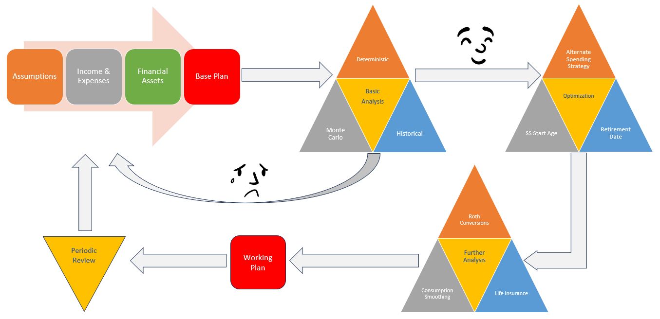
This user manual will help you understand how Pralana is organized and how to get the most value from its extensive capabilities. Most users begin by creating a base plan, then iteratively refine it—examining alternatives, exploring “what-if” scenarios, and optimizing decisions—until they arrive at a working plan. From there, your plan can be easily revisited, reviewed, and refined over time as circumstances, assumptions, or goals change.
The planning process within Pralana follows these steps:
Build – Enter personal and family information, define key assumptions, and provide details about assets, income, and expenses to establish a base plan.
Review & Analyze – Run initial analyses to assess plan viability, including the probability of not outliving your assets.
Refine & Optimize – Adjust inputs, explore alternatives, and apply optimization tools to arrive at your working plan.
Revisit – Periodically return to your plan to update assumptions, reflect new information, and re-analyze outcomes.
Subscription Levels
Pralana offers three subscription types for different needs. Each subscription supports one or more plans. Plans may include up to three scenarios test alternative income, expense, account growth and other assumptions.
Platinum: supports a single plan
Platinum Family: allows you to create up to 5 separate plans for yourself and others.
Platinum Pro: adds plan-management features for financial advisors and is offered in tiers supporting 25, 50, and 100 simultaneously active clients.
Key Features
Pralana’s depth of features and calculation transparency distinguish it from many other financial planning tools.
Sources of Income:
Employment, pensions, Social Security, annuities, windfalls, and miscellaneous income.
Social Security benefits, including spousal and survivor benefits, are calculated based on your start ages and your benefit at your full retirement age.
Expenses:
Personal property and rental property, including user-defined operating costs and capital improvements.
Children’s expenses, including college tuition, loans and 529 college savings plans.
Healthcare expenses, including auto-calculation of Medicare premiums and IRMAA, ACA subsidies and support for Health Savings accounts.
Charitable giving, including QCDs from your IRAs and inherited IRAs.
User-defined expenses. Each may be categorized as essential or non-essential and you may specify different inflation assumptions and other parameters.
Loans: Purchase, refinance, home equity loans and HELOCs on personal and rental property.
Investment loans as well as personal loans made by you to others.
All loans support interest-only periods, additional principal payments, early payoff, and user-defined tax deductibility of interest.
Insurance:
Term and cash-value life insurance modeling.
Accounts:
Eleven types of accounts including cash, taxable, tax-deferred (401k, IRA, etc.), Roth IRAs and inherited traditional and Roth IRAs.
Calculation of RMDs for tax-deferred and inherited traditional IRAs.
Scheduled account transfers of funds between accounts as well as transfers of appreciated assets to external organizations.
User-defined account withdrawal order to cover cash shortages.
Simple and advanced portfolio growth modeling using rates of return by account or user-defined asset classes. Seven options to categorize how growth in taxable accounts is taxed.
Analysis and Optimization Tools:
Monte Carlo and historical analyses provide a way to test scenarios using randomized or historical rates of return.
Historical sequence testing, allowing you to evaluate your plan against some of the worst market periods on record.
Roth conversion planning and optimization, including constraints by user-specified tax brackets, capital gains brackets, IRMAA thresholds, and ACA Federal Poverty Level multiples.
Social Security start age optimization.
Earliest safe retirement date analysis.
Seven variable spending strategies: consumption smoothing, constant spending, fixed % spending, fixed % spending with floor & ceiling, Guyton-Klinger, target % adjustment and actuarial. These strategies dynamically adjust spending during retirement based on portfolio performance.
Results Views:
Interactive charts illustrate projected income, expenses, savings, net worth, taxes and more.
Rich tabular projections, including detailed year-by-year income, expense, cash flow, balance sheet, and asset allocation views.
Pralana’s “Metric MRIs,” available for tabular projections and tax forms, provide transparency by showing how key values—such as Social Security income, account balances, healthcare costs, and Roth conversions—are calculated.
Report generation and export to Excel and PDF, enabling printing and sharing of your plan.
Tax Forms Supported by Pralana:
Pralana estimates your Federal, state and local tax liability each year and shows you a representation of the forms listed below. More forms may be added over time.
1040 U.S. Individual Income Tax Return Federal forms and schedules: 1040 Personal Exemption Worksheet 1040 Schedule 1 Additional Income and Adjustments to Income 1040 Schedule 2 Additional Taxes Schedule A Itemized Deductions Schedule D Capital Gains and Losses Schedule E Supplemental Income and Loss 4797 Sales of Business Property 6251 Alternate Minimum Tax 8582 Passive Activity Loss Limitations 8606 Nondeductible IRAs 8812 Credits for Qualifying Children 8960 NIIT 8962 ACA Premium Tax Credit 8995 QBI Deduction |
Unrecaptured Section 1250 Gain Worksheet Federal worksheets: Schedule A Home Mortgage Interest Worksheet Schedule A Itemized Deductions Worksheet Schedule D Capital Loss Carryover Worksheet Schedule D Tax Worksheet 1040 Qualified Dividends and Capital Gains Worksheet Pub 915 Figuring Your Taxable SSI Benefits 6251 AMT Exemption Worksheet 8812 Credit Limit Worksheet A State and local forms: State Generic Tax Return Local Generic Tax Return GA Form 500 Schedule 1 Page 2 Retirement Income Exclusion GA Form 500 Schedule 1 Page 3 Military Retirement Income Exclusion |
|---|---|
Scenarios in Pralana
Pralana is a powerful decision-making tool that lets you model different assumptions and evaluate their long-term impact. In Pralana, a ‘scenario’ is a complete set of assumptions, income sources, and expenses. Pralana allows you to define up to three scenarios and compare their results.
On most pages, only inputs or projections for one scenario is visible at a time. You select the active scenario using the radio buttons near the top of the page. This lets you enter different values for the same fields across scenarios—such as life expectancy, inflation, asset allocations, income streams, and expenses.
All scenarios share a common set of key plan-level input such as demographic information (your name, date of birth) and initial account balances.
Income and expenses as well as asset allocations and rates of return may be defined differently for each scenario.
Results are shown graphically and in detailed tables to help you compare possible outcomes. Most tabular projections provide the option to compare metrics from two or more scenarios.
Create an additional scenario: go to Build > Scenario Assumptions > Add/Delete Scenarios and enter a name and description.
The new scenario will be created with a few values copied from Scenario 1. The scenario radio buttons will then appear on all input pages, allowing you to select which scenario to modify, view and run analyses.
Pralana provides tools to help you compare your scenario inputs and projections as well as copy inputs between scenarios.
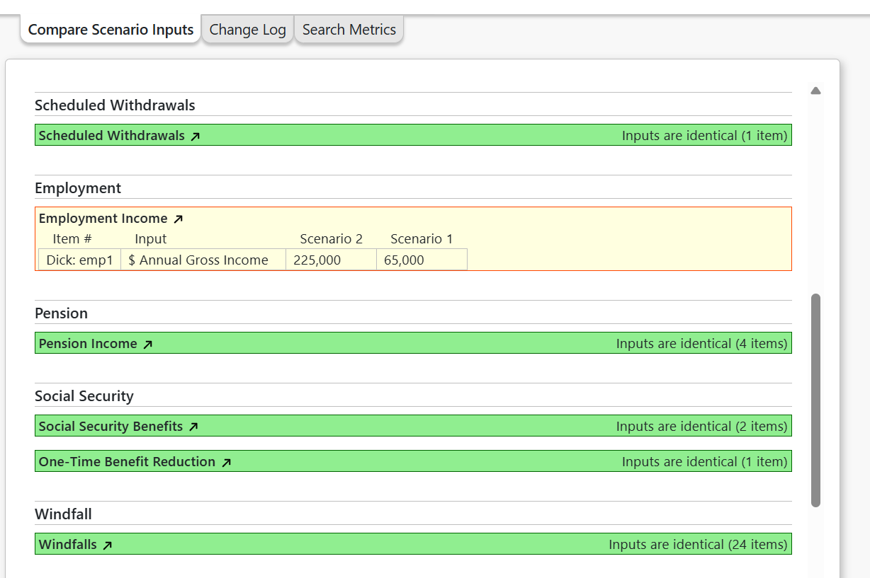
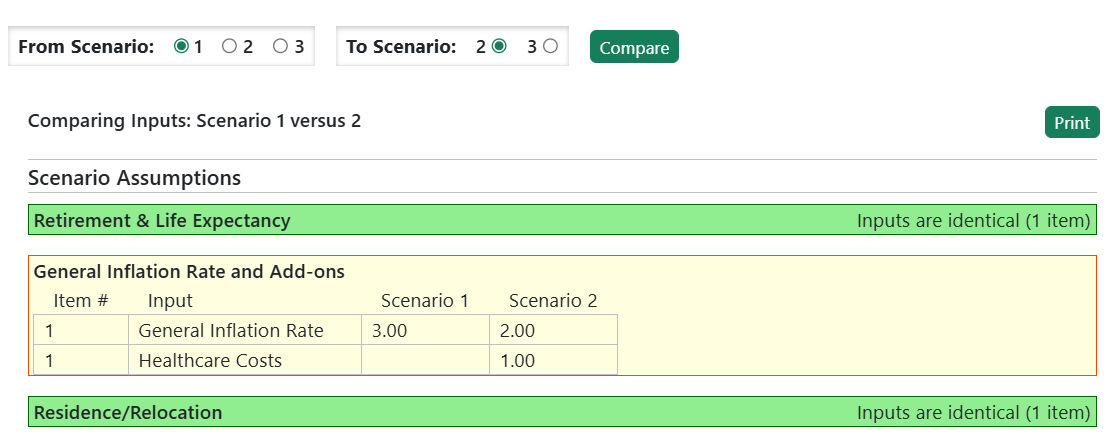
Compare Scenario Inputs
This page shows a comparison of the inputs for two selected scenarios, highlighting differences. It is organized by input page, with links to those pages.
Compare Scenario Results
This page, available at Review > Graphical Projections, includes a chart and table that shows projection of key metrics for the selected scenarios. Controls on this page:
Compare to Scenario: If your plan has more than one scenario, select the scenario(s) you want to compare to the currently active scenario.
Chart Metric: Select from one of several metrics to display on the chart.
Table Metric: Select ‘Same as Chart’ to have the table show the chart data, highlighting differences in the metric values by year. Select ‘All’ to have the table show all available key metrics.

Scenario Analysis Comparisons
This page compares the results of the Monte Carlo or Historical analysis for each scenario for which you have run the analysis.
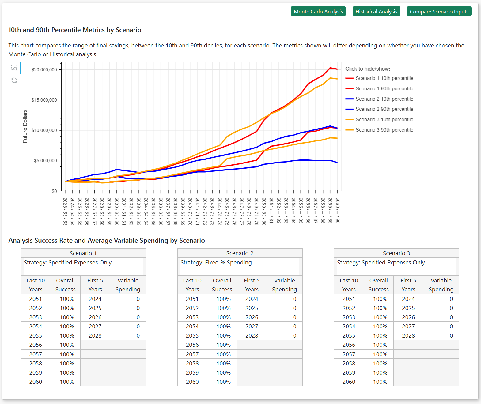
The graph shows the 10th and 90th percentile values from all three scenarios, color. The entire set of colored bands (like on the Run Analysis page) are not shown because the results from one scenario would obscure the results from the others. Here is the key to understanding this graph: the 10th and 90th percentile lines from a given scenario are of the same color and the space between them is all the blue bands shown on the Run Analysis page would be located. So, by comparing this “transparent” envelope from one scenario with that of another scenario, you can get a good sense of the relative success rates of those scenarios. With that said, this graph can display either savings or spending results as specified by the radio buttons at the top of the page. You may select to show the data in future or today’s dollars. Savings may be shown in effective or absolute dollars.
The table beneath the graph contains tabular success rates for the final 10 years of all three scenarios and variable spending for the next 5 years.
In the case of a scenario that models a shorter lifespan than the other scenarios, you will observe that the time axis extends beyond the death year and the savings and expense values drop to zero in those final years.
Things You Need to Know
The Welcome page (Home > Welcome) contains a quick overview of Pralana’s navigation, icons and links and various other things you need to know to use the site effectively.
Icons and Scenario Selection Control
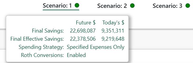
Scenario Status
Almost every page shows the status of each scenario. By hovering your cursor over these icons, a pop-up box shows key information about the scenario. If the portfolio is in positive territory, the scenario icons will be green; otherwise, they will be red. The dots will appear to spin which the scenario is recalculating.
Pralana models up to three scenarios simultaneously but in most cases the inputs and outputs from only one of these scenarios will be visible at a time. You can select the active scenario via radio buttons like these:
 .
.
Site Icons and Links
Below is the guide from the Welcome page:
Scenario Snapshot / Baseline
 icon at the top of the page
to save a snapshot of the active scenario’s projections to ‘baseline’.
The baseline contains key results metrics, by year, for the scenario.
After setting the baseline, you may continue editing the scenario’s
inputs. To see how those edits have altered the scenario’s
projections, go to Review > Graphical Projections > Current vs
Baseline.
icon at the top of the page
to save a snapshot of the active scenario’s projections to ‘baseline’.
The baseline contains key results metrics, by year, for the scenario.
After setting the baseline, you may continue editing the scenario’s
inputs. To see how those edits have altered the scenario’s
projections, go to Review > Graphical Projections > Current vs
Baseline.Currently, Pralana saves only one snapshot/baseline of a scenario. When you set the baseline again, the baseline data is updated with the current scenario results.
Dynamic Number of Income, Expense, and Other Items
Pralana allows you to add and delete scenarios, income and expense items, asset classes, time periods, expense categories, and many other items. Each input form will display your current items and provide a “new” row or column through which you create additional items. To create a new item, just populate the “new” row or column, where the required inputs appear with a light blue background. Once those fields have been populated, the new item will immediately be added to the input form, the new label removed, and may continue filling in the remaining fields. To delete any line item, just click the red X at the right of the input’s row, (or bottom, if the fields are in a column).
The More > Resources > Max Number of Items page shows the maximum number of items you can define for each income, expense and other types of inputs. It also shows whether these inputs are plan-wide (apply to all scenarios), scenario-specific, property-specific, etc.
Pralana Supports a Single Browser Tab per User
Please be aware that Pralana supports only a single browser per user; if you create a duplicate tab in your browser and then attempt to access different views into Pralana simultaneously, you will encounter errors as it is not currently designed to support this mode of operation. Please refrain from this and restrict your usage to a single tab.
Tabular Projections
Pralana includes many tabular projections which are tables showing the projected values of metrics (in columns) by year (in rows). Tabular projections have these features:
Scenario selector: If your plan has more than one scenario, use this control to change the active scenario and update the tabular projection data.
Future $ or Today’s $ selector: You may select whether the values are shown in Future $ or Today’s $. See the “Future Dollars vs Today’s Dollars” below for more information.
Show Empty Columns: When checked Pralana will display all available columns, whether applicable or not. The default is to hide empty columns. Note: a few columns cannot be hidden including loan payments and interest on loan amortizations.
Compare to Scenario: Many tabular projections let you compare the active scenario to other scenarios, if your plan has more than one scenario. See the “Compare Scenario Metrics” section below.
Create PDF: Clicking this button will create a PDF of the tabular projection and open it in a new browser tab where you can view and download it.
Export to Excel: Clicking this button will export the tabular projection to Excel and prompt you to save the Excel file on your computer.
Column Heading Tooltips: Many column headings have an explanatory pop-up text box that will appear when you hover the cursor over the [i] symbol.
Gray First Row: For tabular projections that include account balances, property values, or loan balances, a gray row is shown at the top of the table to display the starting values as of December 31 of the year prior to your plan start year. This row serves as a reference and reflects the values you entered. All subsequent rows generally show year-end values. For example, if your first plan year is 2026, the balances shown in the 2026 row represent values as of December 31, 2026, after accounting for growth and any credits or debits during that year.
Totals Row: When displayed in Today’s $, most tabular projections will display a Total row at the bottom which will include totals for income, expenses, account growth and other metrics when meaningful. Totals are not shown for percentages (e.g. marginal tax rates) and end-of-year account balances, net worth, property values and loan balances.
The total row is never shown when viewing the table in Future $ because totals of Future $ are meaningless and misleading.
Example: You receive a $1million non-taxable windfall, in Future $ in 2026 in scenario 1 and in 2046 in scenario 2.
In Future $, the total windfall received is the same: $1million. But in Today’s $, the value received in 2026 is worth significantly more than the value received in 2046, reflecting the loss of purchasing power due to inflation over time.
Compare Scenario Metrics
When your plan includes multiple scenarios, certain tabular projection pages allow you to view results from two or three scenarios side-by-side. These pages will display a “Compare to Scenario” selector at the top. You can enable or disable other scenarios to add or remove their metrics from the table.

When additional scenarios are selected, Pralana prefixes each column with its scenario label (e.g., S1, S2, S3), as shown below. Values that differ from the first (baseline) scenario are highlighted visually.
If a comparison scenario differs from the first scenario, its values are highlighted with a yellow background.
If three scenarios are shown and all three values differ from each other, the third scenario’s values are highlighted with a blue background.
Small symbols (●, ◆) may also appear next to differing values to make differences easy to spot.
This visual formatting helps you quickly identify differences.

Future Dollars vs Today’s Dollars
Pralana enables you to view its tabular and graphical projections in terms of either future dollars or today’s dollars, as specified by radio buttons like this:

Pralana uses the term “today’s dollars”, but it is technically identical to the term “present value” of a future income, expense, or account balance. See Appendix 2 – Future vs Today’s $ for more.
Income Examples
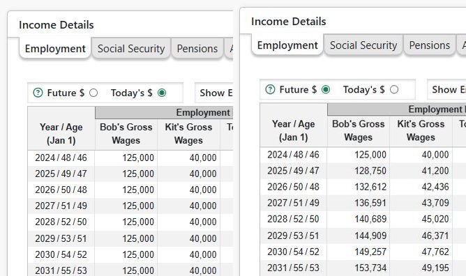
Now, let’s look at some income-related examples in Pralana. In the shot below, inflation is 3%. Bob earns $125,000 with a 3% annual COLA and Kit earns $40,000 with a 3% annual COLA. The shot on the left shows this in terms of today’s dollars and the shot on the right shows it in terms of future dollars. They have expenses of $75,000 that they expect to increase at the rate of inflation, or 3%. In terms of today’s dollars, both Bob’s and Kit’s incomes are flat and so are their annual expenses. Meanwhile, note that their Total Savings is increasing each year, thus signifying that its present value and its buying power is increasing each year.

Below is a similar example, except that in this case Kit has a fixed income with no annual adjustments. As you can see, in terms of today’s dollars her income is diminishing every year even though it is constant in terms of future dollars. This income stream is losing buying power every year. Meanwhile, Bob’s income is keeping up with inflation and maintaining its buying power.

Now, let’s take a look at a different example where Dick and Jane are retired and have no income. They do still have expenses, so they have a negative cash flow each year. The shot on the left shows their balance sheet in terms of today’s dollars, and the shot on the right shows their balance sheet in terms of future dollars. You can infer from this that the buying power of their savings is decreasing each year but that is not evident when looking only at the balance sheet on the right, thus illustrating the benefit of seeing the data in terms of today’s dollars, or its present value.
Expense Examples
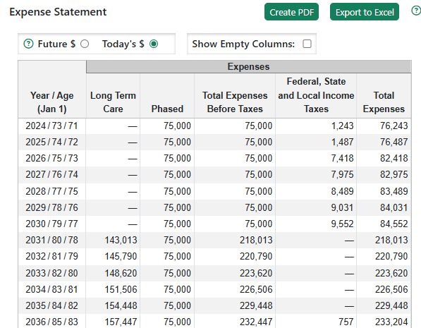
Now let’s look at some expense-related examples. In the shot below, you can see that general inflation is 3% and there are no add-on increases for healthcare, long-term care, college, etc. We have specified phased expenses of $75,000 starting in 2024 and LTC expenses of $125,000 starting in 2031. Here is a shot showing those projected expenses in terms of today’s dollars.

Now let’s include 2% LTC-specific inflation on top of general inflation, as you can see here:

Now let’s see what effect this has on the projection of expenses:

In contrast to the case with no LTC add-on inflation, this case does have some LTC add-on inflation and, therefore, LTC expenses are increasing in terms of today’s dollars while Phased expenses remain constant as in the prior example. This is the expected result of an expense that increases faster than the general inflation rate since that rate is the basis for converting future dollars into today’s dollars.
Unscheduled Withdrawals and Iterative Tax Calculations
Pralana performs detailed income tax calculations and includes those taxes in annual expenses which are subsequently used to determine annual cash flow. When that cash flow is negative, it results in a subsequent unscheduled transfer (i.e., a withdrawal) from one or more of the taxable savings, tax-deferred savings or Roth savings accounts, depending upon the withdrawal priorities specified by the user on the Financial Assets/Management page and the balances of those accounts.
Any such unscheduled transfers from tax-deferred accounts are a taxable event; however, the taxes for the year in question will have already been calculated and iterative tax calculations are required to properly determine the total taxes for this case. Pralana is designed to do these iterative calculations but that capability is not enabled in the releases to date. The reason for this is to enable direct comparisons to PRC2023 and PRC2024 (Excel) which do not perform iterative tax calculations. Consequently, for now, those transfers are treated as ordinary income in the next year, and that will be reflected in the next year’s AGI just as they are in the Excel tool.
Any such unscheduled transfer from taxable savings that results in long term capital gains is a taxable event and is handled the same as unscheduled transfers from tax-deferred savings.
Long term effects of this design simplification on the accuracy of Pralana’s projections have been studied and they are minimal; however, this may affect the optimization of Roth conversions in the near term.
Best Practice for Using Pralana
Pralana is a powerful and flexible planning tool, and it is best approached as an iterative process rather than a one-time exercise. This section provides a recommended workflow to help you build, analyze, and refine your plan without becoming overwhelmed. Some terms and features mentioned here are explained in more detail later in the manual; for now, focus on the overall progression. You can return to this section as your familiarity with the tool grows.
1. Start Simple with Quick Start
Begin by using Quick Start to create an initial version of your plan. Navigate to Build > Get Started > Quick Start and enter approximate information about your income, expenses, assets, and assumptions. At this stage, precision is not important—your goal is to establish a reasonable baseline.
After completing Quick Start, visit the Build > Income, Build > Expenses, and Build > Financial Assets pages to see how your inputs were translated into detailed entries. Then review the results on Review > Tabular Projections to gain a basic understanding of what the projections are showing.
2. Build Out the Details
Next, return to the Build pages and add more detail to your income sources, expenses, and assets. If you have not yet started Social Security, select start ages for yourself and your spouse—you can refine these later.
You may want to periodically set/update the baseline so you can see how changes affect the scenario results.
As you add detail, review the associated income or expense projection on the input page or return to Review > Tabular Projections to confirm that the overall results align with your expectations. At this stage, focus on understanding the deterministic projections before moving on to more advanced analyses.
3. Assess Risk with Monte Carlo Analysis
Once your deterministic results make sense, run a Monte Carlo analysis using the default assumptions. This analysis helps you understand the range of possible long-term outcomes and the likelihood that your plan remains viable.
If the projected success rate seems unacceptably low, consider adjustments such as:
Delaying retirement
Changing Social Security start ages
Reducing spending
Adding part-time work in retirement
Modifying your investment strategy
You can freely iterate between the Build, Review, and Analyze sections as needed. If desired, you can also explore different assumptions for market volatility directly on the Analyze > Monte Carlo Analysis page.
4. Explore Historical Outcomes
After reviewing Monte Carlo results, consider running a Historical analysis. This allows you to see how your plan would have performed under actual historical market and inflation conditions. You may also test specific historical sequences—such as starting in 1965, which represents one of the most challenging periods for retirees.
5. Optimize Key Decisions
With a viable plan in place, you can begin using Pralana’s optimization tools:
Social Security Optimization to evaluate alternative claiming strategies
Earliest Safe Retirement Date Analysis to determine when retirement becomes feasible with an acceptable probability of success
Variable Spending Strategies to model how discretionary spending might adjust in response to portfolio performance
Pralana supports up to three scenarios per plan, making it easy to compare strategies side by side.
6. Refine Tax and Roth Conversion Strategies
Roth conversion planning depends on many factors, including asset allocation, tax-deferred balances, tax brackets, ACA subsidies, and IRMAA thresholds. For this reason, it is generally best to explore Roth conversions after the rest of your plan is largely established.
Using Pralana’s Roth conversion tools, you can set constraints and allow the system to determine conversion amounts that seek to improve long-term after-tax outcomes. You may also specify specific conversion amounts, when needed.
7. Maintain and Revisit Your Plan
At this point, you have established a working plan. From here on, Pralana becomes an ongoing decision-support tool. As assumptions change, life events occur, or actual market returns replace estimates, you can revisit the Build pages, update your inputs, and re-run analyses to keep your plan current.
Updating your plan’s start year: See Appendix 1: How do I update my plan at the start of a new year? for tips on updating your plan at the start of each year. This information is also available in Pralana Online at More > Resources > FAQ and in the Pralana forum.
Structure and Navigation
Pralana is organized into several major, interrelated sections that are accessible from the fixed navigation bar at the top of every page. Depending on your subscription level, these sections include Advisors, Build, Review, Analyze, and More.
The Advisors section (available with a Platinum Pro subscription) enables financial advisors to create, manage, and maintain plans for multiple clients.
The My Plans section (available with a Platinum Family subscription) lets you see and manage multiple plans.
The Build section is where you create and modify your plans by entering assumptions, assets, income, expenses, and other inputs.
The Review section provides detailed outputs, including tabular projections and charts, and allows you to generate PDF reports and compare scenarios.
The Analyze section contains tools for analyzing and optimizing your plan, such as Monte Carlo and historical analyses, spending strategies, and optimization features.
The More section provides access to supporting information, including guidance on using the tool and release notes.
Hovering over top-level menu items reveals a submenu with links to related pages, organized by function, as illustrated in the screenshot below.

Advisors
The Advisors section contains two subsections:
Advisor Profile, where you can specify your name, certifications and contact information for Reports produced for your clients.
Client Plans, where you can add, manage and delete plans associated with multiple clients. Client Plans has a tab ‘Plan Adoption Log’ that shows the history of plans adopted by a client.
The Advisor link and subsections will only be visible to Platinum Pro users.
Home
The Home menu contains three pages:
Welcome: provides useful information for new subscriber about using Pralana and how to get started building their plan.
Features: shows key features of Pralana.
Dashboard: landing page when logging in. It contains summary information about your plan and scenarios as well as charts and tables showing various plan projections.
Build
The Build section is where you provide the detailed inputs to establish your financial plan, and it contains these subsections:
Get Started - Begin defining your financial plan:
Quick Start, My Family, Scenario Assumptions, Import PRC Excel Export File
Financial Assets - Identify your financial accounts, characterize your portfolio, and define personal and investment loans:
Management, Accounts, Portfolios, Scheduled Withdrawals, SEPPs, Personal Loans and Investment Loans
Income - Define your sources of income:
Employment, Pensions, Social Security, Windfalls, Annuities and Other Income
Expenses - Define your expenses:
Personal Property, Rental Property, Children, Healthcare, Long-Term Care, Charity, Miscellaneous, Phased, Term Life Insurance and Cash Value Life Insurance
Review
The Review menu contains these items that provide a detailed output of your financial plan:
Tabular Projections: detailed tabular projections for your scenario(s), including Income, Expense, Cash Flow statements, Balance Sheet and Tax Summary with many supporting tables.
Graphical Projections: charts showing projected savings and net worth, taxes and other graphical projections
Reports: Plan Inputs Report, Plan Results Report (both of which will create PDFs) as well as Tax Forms and related tax information.
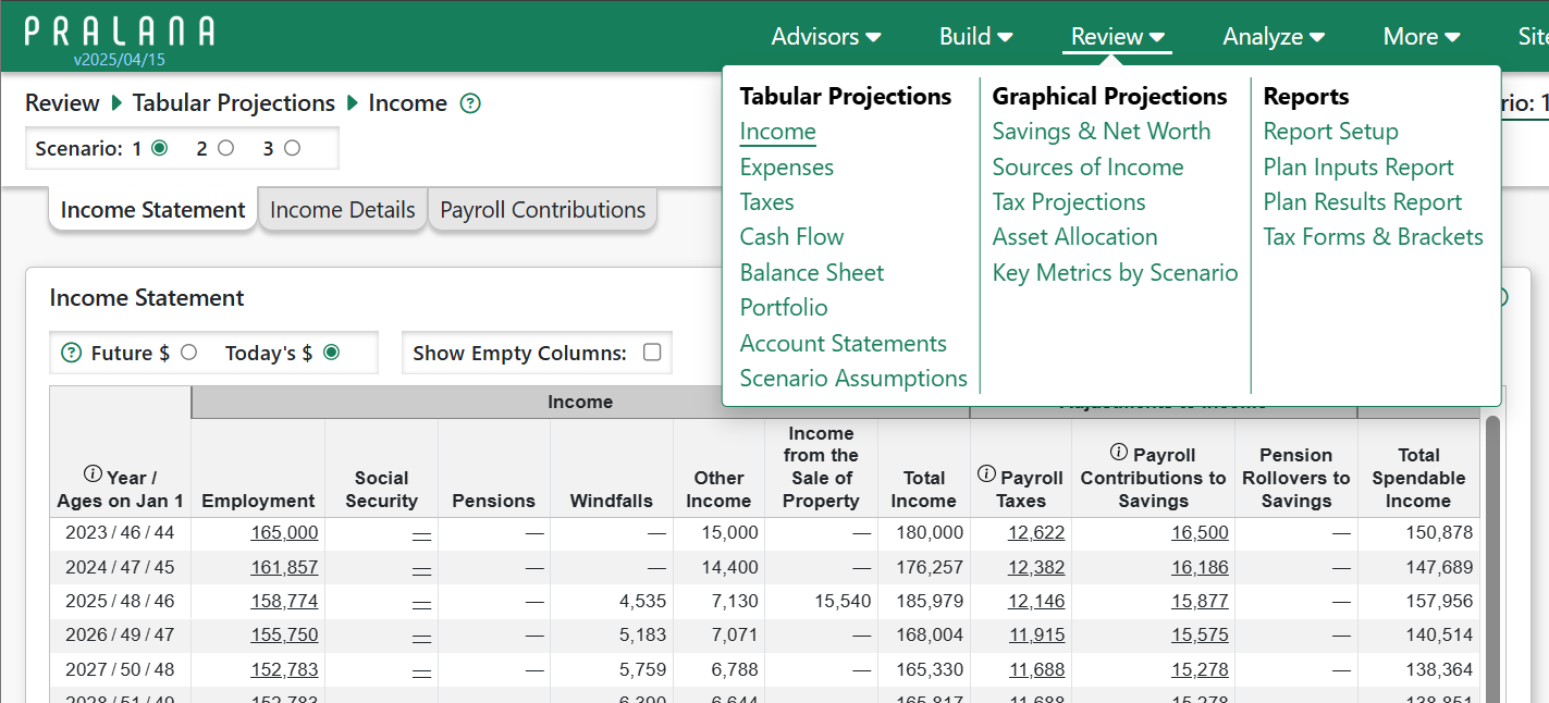
Here is a screenshot of the Review pop-up menu:
Analyze
The Analyze section contains these subsections:
Monte Carlo Analysis: allows you to run and see the results of a Monte Carlo analysis of each scenario.
Historical Analysis: allows you to run and see the results of a Historical analysis of each scenario.
Spending Strategies: explore various alternate spending strategies, including Consumption Smoothing
Roth Conversions: define and optimize Roth conversions.
Optimize Social Security Start Age: determine the optimum Social Security start age for yourself and, if married, a spouse.
Optimize Withdrawal Priorities: an analysis to optimize withdrawal priorities among your various accounts when scenarios have cash shortages.
Earliest Safe Retirement Date: finds the earliest retirement date that yields a 90% probability that you will not outlive your money.
Here is a screenshot of the Analyze pop-up menu:

More
The More section contains links to other Pralana features which will evolve over time.
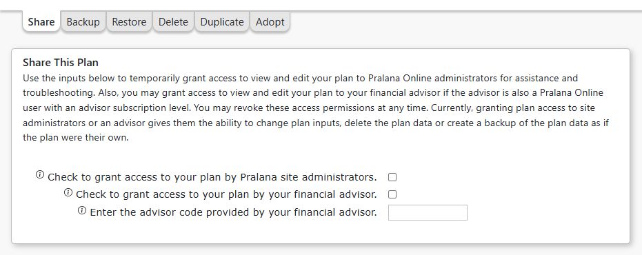
Manage My Data: provides access to features which allow you share your plan, backup, restore and delete your data from Pralana.
Alerts: shows various general site announcements and plan-specific messages generated by Pralana to make you aware of potential issues with your data. It may also contain information about known, unresolved bugs and site outages.
Feedback: shows your feedback and responses from the Pralana team
Release Notes: Shows recent past and pending future site change.
Resources pages for:
General Resources contains credits and acknowledgements as well as financial planning resources.
FAQ has answers to frequently asked questions.
How Do I… This section links to Appendix 1, providing brief explanations for common tasks and frequently asked questions about using Pralana.
PRC Excel vs Online summarizes differences between Pralana Gold (Excel) and Pralana Online.
Privacy Notice
Terms of Use
Other items such as site preferences and beta features.

Features in the More Menu
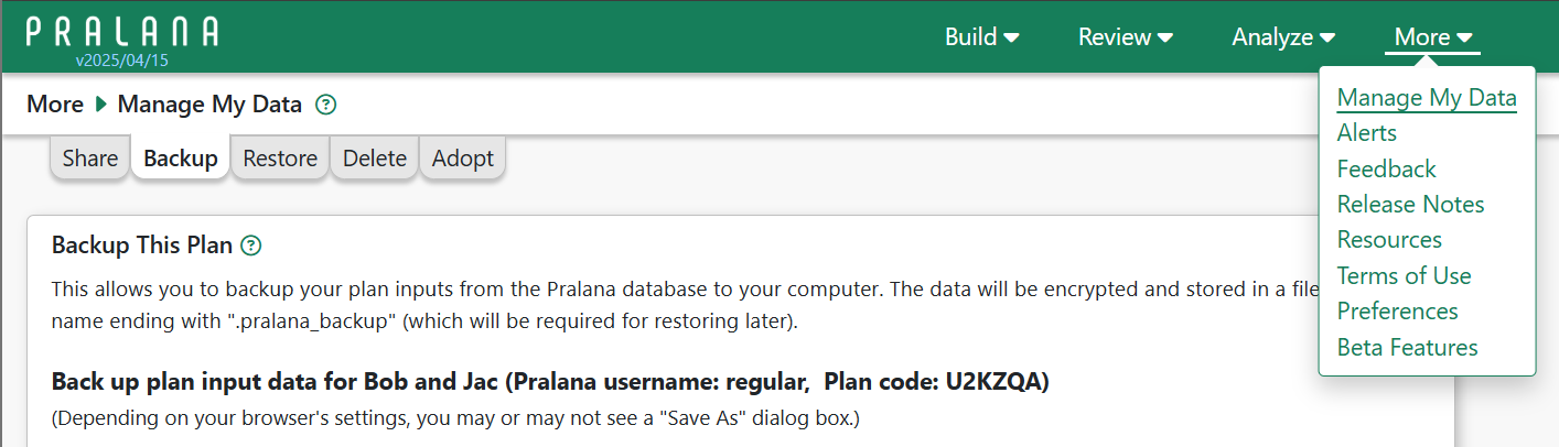
Manage My Data
Selecting Manage My Data from the More menu will take you to a page with six tabs, as shown here:
See the Data Security section for information about what data is provided to Pralana and how it is secured as well as best practices you can use to protect your data.
Backup This Plan
You may use this feature to extract and download your Pralana plan input data to your local computer. The downloaded file will be encrypted and may contain security measures to prevent unauthorized use by others or use in violation of the Pralana Terms of Use for your subscription level. The backup is intended for short term use. See notes on the Backup page and the limitations below in the Restore section, below.
Restore Plan from Backup
You may use this feature to restore your Pralana plan using a previously downloaded Pralana backup file. We will make reasonable, best efforts to maintain backward compatibility for restoring backup files as Pralana is updated over time. The financial projections made by Pralana using a recovered backup file may differ from the projections made at the time the backup was made due to changes in tax parameters and changes to the calculations. You will be notified when restoring if the plan’s final year savings for each plan scenario match or differ from the corresponding amounts at the time the backup was created. See Appendix 4 – Restore from Backup Reference for more information about restoring from backup for the various subscription levels.
Delete This Plan
At any time, you may use the Delete feature to immediately, permanently and irrevocably remove your plan data from the Pralana database. Your plan inputs will be deleted and replaced with a generic plan for a fictitious ‘Dick’ and ‘Jane’. See the Data Security section for more information. You may request the site administrators delete your Pralana username/account by emailing us at mail@pralanaconsulting.com.
Duplicate This Plan
Applicable only to Pralana Pro users, the Duplicate function creates a new plan identical to the currently selected plan. This enables you to establish a “template plan” as a starting point for creating new client plans.
Adopt a Plan from Someone Else
The Adopt function enables you to adopt a plan created by another user, transferring ownership of that plan. For example, a financial advisor may create a plan for a client and then allow the client to adopt the plan. Or a person may create their own plan, then allow their financial advisor to adopt the plan (rather than temporarily sharing the plan). In either case, both client and advisor must have a Pralana subscription.
To adopt a plan, the current plan owner provides the plan code and a secret word to the recipient who enters that info on the Adopt page and simply clicks the ‘Adopt Plan’ button. While there are well over 1 billion possible plan codes, the secret word requirement adds an extra layer of security. The adoption process effectively changes the ownership of the plan and only the owner of a plan can delete that plan. Advisors can never own more plans than their Pralana subscription supports.
Important:
If the person adopting the plan is an individual user, the adopted plan will irrevocably replace the person’s existing. If the recipient is an advisor, adopting a plan will simply add the newly adopted plan to the advisor’s list of plans.
The existing owner of the plan will no longer have access to the plan, after it is adopted. If the existing owner is an individual user (not an advisor), a new plan with default inputs will be created for the existing owner.
The existing owner may choose to create a Pralana backup of the plan before providing the adoption information to the recipient. This back up may be later restored (see Restore for important information).
Tools
Compare Scenario Inputs
If you have at least 2 scenarios, this feature lets you compare the inputs between 2 of your scenarios. It will show you the categories of inputs that are the same and, if different, which items are different. Optionally, you may choose to see differences only. This is useful if the 2 scenarios were identical and you subsequently made changes. It highlights the changes.

Change Log
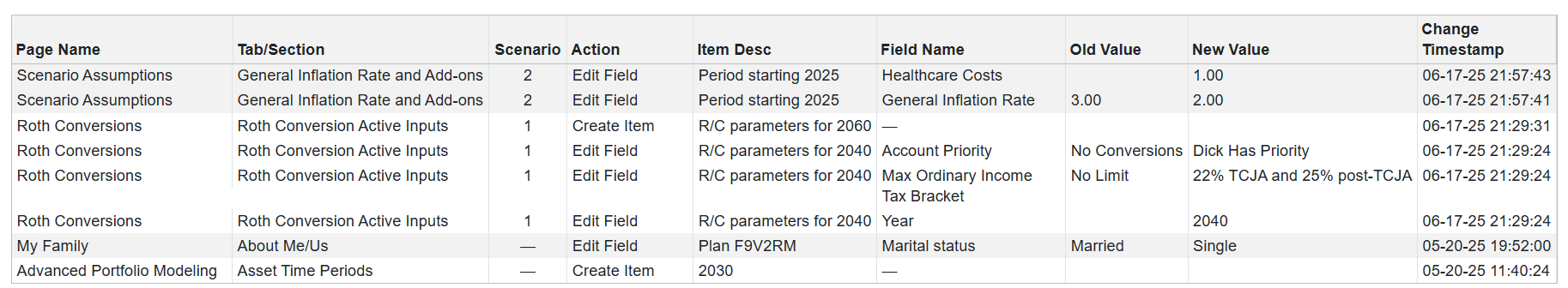
The Change Log shows the most recent edits to your plan. Use this to look back to see old and new values for each edit. The log will periodically be pruned to contain only the most recent 100 edits. Certain actions, such as restoring a plan from backup or copying or deleting a scenario may delete log items prior to that action.
Search Metrics
This feature allows you to do a keyword search of the column names in all tabular projections. The results will show a list of matching columns, with the associated Page Name, Column Name, and other useful information along with a link to that tabular projection.
Alerts
Pralana generates user alerts to make you aware of announcements from
the develop, announcements regarding the completion of imports from
Pralana Gold and any related import errors, and error conditions that
have been detected while running the model on your data. Whenever one or
more alerts, other than ‘Success’ (green) are present with, you will see
one of these icons 

 (‘Info’, ‘Warning’,
‘Error’) in the status bar. The color represents the highest alert
severity level, if there are multiple alerts. To access your alerts, you
can click that icon, or you can click “Alerts” in the More menu.
(‘Info’, ‘Warning’,
‘Error’) in the status bar. The color represents the highest alert
severity level, if there are multiple alerts. To access your alerts, you
can click that icon, or you can click “Alerts” in the More menu.
The Alerts page organizes alerts by category and within category by scenario, if applicable. As with the icon in the status bar, the color of the alert indicates the severity: green=success, blue=information, yellow/orange=warning, red=error. The categories are:
General alerts applicable to all users. Usually these announce new features or provide other important site news.
Plan alerts specific to your plan which may include:
Feedback alerts: Let you know one of your feedback items has been updated by the Pralana staff.
Import alerts: Give you information about an issue encountered when importing data from your PRC Gold export file.
Input alerts: Warn you about an issue with one of your inputs.
Calculation alerts: Warn you about an issue encountered when calculating your scenario projections.
Error alerts: Warn you about an error that has occurred.
Other alerts: Other types of alerts.
Most alerts first appear on either the applicable page or on all pages. You can dismiss alerts by clicking on the circled ‘x’ icon in the top right corner. Dismissed alerts will appear on the Alerts page where you can click the circled ‘x’ again to Delete Forever.
Some alerts will re-appear if the condition that created them occurs again. Other alerts will automatically disappear if the condition that created them no longer exists.
Many alerts that affect multiple scenarios and/or projection years will be listed once and the affected scenario(s) and/or year(s) will be listed in the body of the alert.
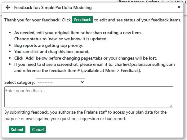
Feedback
Here you can see any feedback items you have created and the staff response. You may edit your feedback item to add an update or change the category or status. Currently, Pralana does not support adding pictures/screenshots to feedback items.
To create a new feedback item, use the Feedback link on the right side of the page header.
Release Notes
This page shows ‘pending’ and recent site changes.
Resources
This page contains useful information about Pralana for our subscribers. Content may be added or changed from time to time.
General Resources
Contains useful information and resources for Pralana subscribers as well as credits for third party data we may use.
FAQ
Contains the answers to frequently asked questions from our subscribers.
Max Number of Items Shows the maximum number of items you can define for each income, expense and other types of inputs. It also shows whether these inputs are plan-wide (apply to all scenarios), scenario-specific, property-specific, etc. ~~~~~~~~~~~~~~~~~~~~~~~~~~~~~~~~~~~~~~~~~~~~~~~~~~~~~~~~~~~~~~~~~~~~~~~~~~~~~~~~~~~~~~~~~~~~~~~~~~~~~~~~~~~~~~~~~~~~~~~~~~~~~~~~~~~~~~~~~~~~~~~~~~~~~~~~~~~~~~~~~~~~~~~~~~~~~~~~~~~~~~~~~~~~~~~~~~~~~~~~~~~~~~~~~~~~~~~~~~
How Do I…
Contains user manual links to commonly discussed retirement topics and how to address them in Pralana. This content is also included in Appendix 1 below.
PRC Excel vs Online
For subscribers of Pralana’s Excel-based products, this discusses some of the differences between PRC Excel and Pralana Online.
Feature Voting
Allows subscribers to cast up to 6 votes for a short list new features to help the Pralana team prioritize these features. There are many more feature and usability requests, not listed on this page, that may also be completed over time. Note: Feature Voting may be moved to the Tools page in an upcoming release.
Beta Features
This page may provide access to features for testing and feedback.
Getting Started
If you were a PRC2023 or PRC2024 Gold user, you can initialize Pralana by importing a PRC2023 or PRC2024 export file. To do that, go to the Build > Get Started > Import PRC Excel Export File page and click the button. That will bring up a dialog box where you can select that export file from one of the folders on your local computer. Click OK and the upload and import process will be initiated. A pop-up message will appear when it is finished. Once you dismiss that, you should be good to go. The Build pages and subpages are where you will find most of your imported data, so a good starting point would be to peruse those pages to see how your data is represented in Pralana. Once you become familiar with that, you can proceed to the Review pages to examine the tabular and graphical projections generated from your data with the deterministic analysis method. From there you can proceed to the Analyze pages to consider doing further analysis of your plan.
When you are ready to start working on your plan, you can just visit each of the links at the top of every page, moving from left to right, and enter your data. Start with your basic assumptions and then progress to the Build menu to specify your income, expenses, and financial assets. Once those have been entered, you can visit the Review pages to examine tabular and graphical projections generated with your data to see how your plan works going forward.
Quick Start
The Quick Start page is intended to minimize the intimidation factor for first-time Pralana users by making the entry of basic assumptions, financial assets, income, and expenses similar to those of a typical, free retirement calculator. Whatever you enter on the Quick Start page will be automatically populated into the normal Pralana input pages where you can elaborate them with additional detail when you are ready. This page just enables you to get started quickly and easily so you can see what Pralana does with your inputs and see the types of outputs it produces with your data.
So, if you are a first-time user of Pralana tools, we recommend making your initial data entry on this page, then perusing the various Build (Financial Assets, Income and Expenses) pages to see how your data appears, and then visit the Review pages. There, you can see the deterministic projections made with your data, including detailed breakdowns of your income, your expenses, the calculated taxes, and the account balances on a year-by-year basis, on both a tabular and a graphical basis.
As you are ready, you can then start adding more detail to elaborate your plan, and there will probably not be any further need for the Quick Start page, so you can just ignore it; however, its contents will automatically be updated to reflect your subsequent inputs via the normal Build pages.
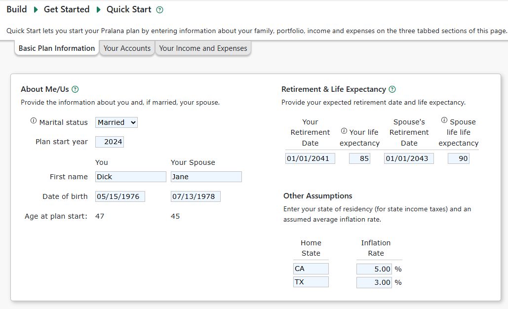
Basic Plan Information
Start by clicking the Basic Plan Information tab which will bring up a page with three simple sections, as shown below. In the About Me/Us tab, simply enter your marital status, your first name and your spouse’s first name (if applicable), your date(s) of birth. In the Retirement & Life Expectancy tab, enter the date you plan to retire from full-time employment and your life expectancy, and then do the same for your spouse, if applicable. In the Other Assumptions section, enter your state of residence and the expected inflation rate. Your inputs in this section will be replicated on the Build > Get Started > My Family and Scenario Assumptions pages.
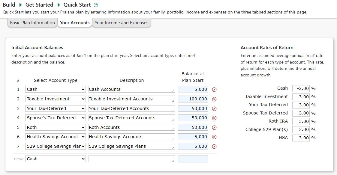
Initial Account Balances
You can click on the Your Accounts tab to tell us about your accounts and their balances as of January 1 in the plan’s starting year. You can specify up to 10 accounts (cash, taxable investment, your tax-deferred, spouse tax-deferred, Roth, 529 college savings plan or health savings account) and for each of these you just need to give it a description and balance at the start of the plan. All the accounts within a given account type will be consolidated and modeled as one by Pralana and hereafter the term “account”refers to the consolidated accounts and not your actual accounts. Inherited accounts are modeled by Pralana, but they are not part of the Quick Start capability. Your inputs in this section will appear on the Build > Financial Assets > Account Initial Balances page. Here is an example:
Account Rates of Return
For each account type, you can then specify the expected average real rate of return (i.e., the return after inflation) in the fields to the right of the account balances fields. Your inputs in this section will appear on the Build > Financial Assets > Simple Portfolio Modeling page.
Your Income and Expenses
Finally, you can click on the Your Income and Expenses tab and define your employment, pension, and Social Security income streams, and your expenses. Windfall income, annuities, and Other sources of income are modeled by Pralana, but they are not part of the Quick Start capability. Likewise, property (personal and rental) expenses, Children’s expenses (including college educations and the associated funding), Healthcare expenses (including ACA and Medicare), are modeled by Pralana, but they are not part of the Quick Start capability. So, do not spend a lot of time trying to model these items accurately via the Quick Start page; maybe just enter some “placeholder” values. You will be able to model them in high fidelity when you are ready to move on to the primary Build pages (i.e., Financial Assets, Income, and Expenses).
Here is an example:
Quick Start Employment Income
You can specify multiple employment income streams for both you and your spouse. For each stream, you can specify the start/stop by either year or age. Then enter the annual amount in terms of today’s dollars and the annual increase amount. If you make contributions to a tax-deferred retirement plan, you can specify those here. Finally, if you receive company matching contributions to your tax-deferred retirement plan, you can also specify those here.
Your employment income inputs will appear on the Build > Income > Employment page. From there, you can add more detail regarding these income streams, if desired.
Quick Start Pension Income
You can specify multiple pension income streams for both you and your spouse. For each stream, you can specify the start by either year or age. Then enter the annual amount in terms of then-year (future year) dollars, along with the expected annual increase amount. Your pension income will appear on the Build > Income > Pension page. From there, you can add more detail regarding your pension income, if desired.
Quick Start Expenses
You can specify your expenses as line items in a simple table. Just enter the expense description, first year and last year (you can leave last year blank if the expense continues indefinitely), and amount in today’s dollars. Your expenses will appear on the Build > Expenses > Miscellaneous page.
My Family
This page contains two sections through which you introduce yourself and your family to the tool: About Me/Us and Children.
About Me/Us
The following items are global in nature and apply to all your scenarios.
Plan Start Year: Enter the year you wish the modeling to begin.
Marital Status: Specify your marital status via the pull-down menu.
Your First Name: Entering your name here will enable Pralana to include it in column headers to help you see the data that is unique to you.
Your Date of Birth: Enter your birthdate in the MM/DD/YYYY format.
Spouse’s First Name: This field will be hidden if a Marital Status of “Single” is selected. Entering your spouse’s name here will enable Pralana to include it in column headers to help you see the data that is unique to your spouse.
Spouse’s Date of Birth: This field will be hidden if a Marital Status of “Single” is selected. Enter spouse’s birthdate in the MM/DD/YYYY format.
Children and Other Dependents
This section allows you to enter your children and others for whom you provide support, their birth year (or the first year you will be providing support) and whether they are dependents for tax purposes.
For those you designate as a dependent for tax purposes, Pralana will, by default, assume tax dependent status for years in which the person is age 18 or younger -or- is in college and under age 24.
Children with gap year(s) between high school and college.
Children in college beyond age 23.
Disabled children or others who qualify as dependents for Federal tax purposes.
Notes:
The “Final Year as a Dependent” field is ignored if you do not check “Is this person a dependent for tax purposes?”
Persons who qualify as your dependents for Federal tax purposes will be assumed to also qualify as dependents for applicable state taxes.
Scenario Assumptions
The first section of this page allows you to specify your assumptions relative to inflation and how it will change over the modeling period.
Add/Delete Scenarios
On this page you can add up to a total of three independent scenarios, each of which has a complete set of assumptions, financial assets, income, and expenses. When you first start using Pralana it will only have one scenario and the active scenario will not be shown on the other input pages (because there’s only one scenario); however, as you add scenarios on this page, radio buttons will become visible on the other pages that enable you to select the scenario you wish to work on (i.e., the active scenario). When you first add a new scenario, it will be initialized to be identical to your first scenario (Scenario 1). You can also use this control to delete a scenario; however, Scenario 1 cannot ever be deleted.
Retirement & Life Expectancy
On this page you can identify the date(s) on which you and your spouse plan to cease full-time employment, or your retirement date. Additionally, you can identify the life expectancy for you and your spouse. Pralana will assume you and your spouse die on the birthday on which the specified Life Expectancy is reached.
The retirement dates you specify here are used by Pralana in four ways:
It identifies the point in time where you MAY lose access to group health insurance premiums. This is used by the healthcare expenses page to assist in determining which time periods are applicable in your case.
It identifies the point in time where withdrawals from tax-deferred and Roth accounts become fair game for maximizing your standard of living and, hence, is used by Pralana’s consumption smoothing algorithm.
It identifies the point in time where non-essential spending (as explicitly specified on the Non-essential and Miscellaneous Expenses pages) can be replaced by variable spending based on your inputs on the Analyze > Spending Strategies page.
It can be used to identify the date on which most income streams can be started or stopped. If you enter the “wild card” character “R” in the start or stop field of an income stream, Pralana will use the retirement date specified here to start or stop that income stream.
If you have already stopped working full time, just enter January 1 of the starting year.
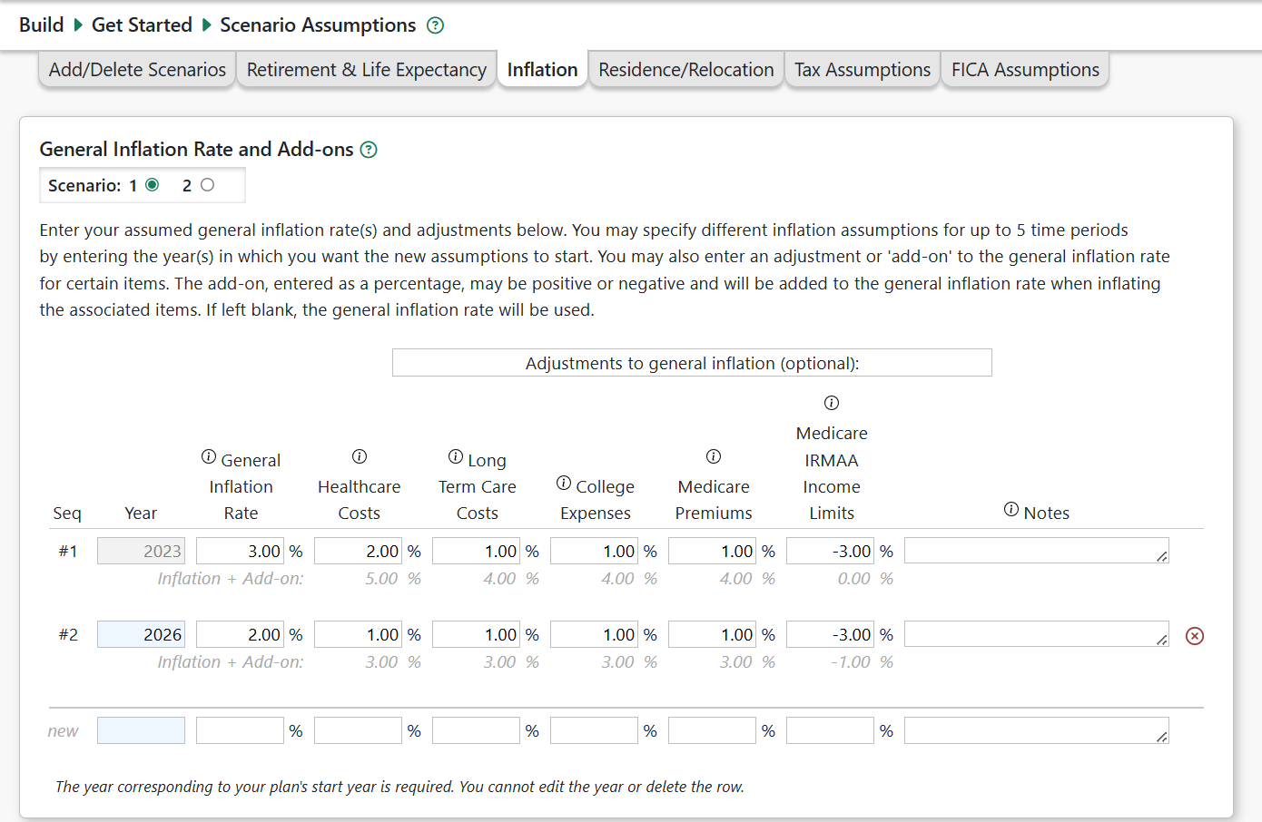
General Inflation Rate and Add-ons
On this page you can identify your assumptions about various forms of inflation, with different values for multiple different periods. Here is a screenshot:
General Inflation Rates
General Inflation Rate for Period 1: This is the general inflation rate that Pralana will use for deterministic calculations and Monte Carlo analyses. This rate will be in effect in the model’s starting year and will continue until and unless a different rate is specified for a second period.
General Inflation Rate for subsequent periods: If you wish to vary the inflation rate over the modeling period, you can do so by clicking entering the rate and start year for subsequent periods in the field labeled “New”.
Inflation Add-ons/Adjustments
You can also add some modifications to the General Inflation Rate. Below each add on, Pralana shows the total of your general rate plus the add-on applicable for that item. We may add additional inflation adjusters in the future.
Healthcare Costs: Healthcare costs will be inflated by the general inflation rate plus any adjustment that you enter here. You may want to factor in an increase in your own healthcare expenses as you get older. Leave blank if you think your healthcare costs will increase at the same rate as general inflation. Note: This adjustment does not affect Pralana’s calculated Medicare premiums which have a separate adjustment described below.
Long-Term Care (LTC) Insurance Costs: Long-term care expenses may be inflated by the general inflation rate plus any adjustment that you enter here. Note that for each long-term care expense you enter, you may choose whether to apply this LTC inflation add-on, your healthcare inflation add-on, or no inflation add-on.
College Expenses: College expenses will be inflated by the general inflation rate plus any adjustment that you enter here. Leave blank if you think college costs will increase at the same rate as general inflation.
Medicare Premiums: Medicare premiums are calculated by Pralana and will be inflated by the general inflation rate plus any adjustment that you enter here. Leave blank if you think Medicare premiums will increase at the same rate as general inflation. Note: This adjustment does not apply to annual insurance premiums and out-of-pocket expenses you enter on the Healthcare Expenses page. Use the Healthcare Costs inflation adjustment, above, for these.
Medicare IRMAA Income Limits: IRMAA income bracket limits will be inflated by the general inflation rate plus any adjustment you enter here. Enter a negative percentage if you think IRMAA income brackets will be inflated less than the general inflation rate, thus causing bracket creep over time.
Residence/Relocation
On this page you can identify your current state of residence and future plans to relocate to another state.
Year: The first row in the table is, by definition, your current state of residence and the year field will always be set to the model’s starting year. If you plan to relocate to a different state in the future, specify the year you plan to move in this field.
State: Pralana performs detailed state tax calculations for your state of residence, as specified here. This field contains a pull-down menu of the 2-letter state abbreviations, and you can just enter a blank if you live in a no-tax state.
Alternate State Tax Rate: State income taxes are particularly difficult to model, with 51 sets of rules (50 states plus the District of Columbia), so it is possible that the model is not always accurate for your case. Pralana state tax calculations ALWAYS use the standard deduction for your state, so that is one potential source of deviation between the model’s tax calculation and your actual taxes. If this algorithm does not seem to be calculating state taxes correctly for your case, you can use the alternative method provided on the Build > Get Started > Scenario Assumptions > Residence/Relocation page. Simply specify a rate that Pralana will multiply by the federal AGI to arrive at an estimate of your state income taxes. If you enter a value in this field, this alternative method will replace the detailed calculations.
Please note: If you do discover that Pralana is producing inaccurate values for the taxes in your state we will always welcome an email to provide us with the details so that we can continue to improve the model.
Local Tax Rate: This is the effective local tax rate in your geographical area. It will be multiplied by your Federal AGI to estimate your annual local taxes.
Tax Assumptions
OBBBA Summary
This page provides an overview of the July 2025 One Big Beautiful Bill Act. Pralana implemented these provisions in July 2025.
Federal Tax Law Settings
The enhanced Affordable Care Act (ACA) subsidies are set to expire at the end of 2025, meaning premiums will rise sharply starting in 2026 unless Congress acts to extend them.
What Are Enhanced ACA Subsidies?
These are expanded premium tax credits introduced in 2021 under the American Rescue Plan (ARP).
They were later extended through 2025 by the Inflation Reduction Act (IRA).
The enhancements made subsidies more generous and expanded eligibility to households earning above 400% of the federal poverty level (FPL)
Year Enhanced ACA Subsidies Expire: This field allows you to specify when Pralana should assume that enhanced ACA subsidies expire. You may set this to different values, by scenario, to see the impact on your ACA subsidies (for otherwise identical scenarios).
Federal Income Tax Rate Changes
Generally, Pralana assumes income tax bracket income limits and many other (but not all) Federal and state tax parameters will increase year-to-year using your general inflation rate. Some Federal and state tax parameters are not inflated. Inflating the ordinary income bracket income limits tends to avoid bracket creep due to income inflation.
Form 1040 line 15,
the Qualified Dividend and Capital Gains Worksheet lines 22 and 24, or
Schedule D Tax Worksheet lines 44 and 46
…as applicable in each tax year. Pralana’s Schedule D line 30 shows which tax calculation method is used.
The ordinary income tax brackets shown on Pralana’s Tax Brackets page are the published rates and will not include your adjustment(s).
FICA Payroll Tax Changes
Pralana can model future increase(s) in FICA payroll tax rates. Use this page to enter a percentage increase in the FICA payroll tax rate, starting in the year(s) you specify. Increase will be handled the same as described for federal income tax increases, describe above.
Import PRC Excel Export File
If you are PRC2023 or PRC2024 Gold user, you can initialize your Pralana plan by importing an export file from PRC2023 or PRC2024. To do this, just click the “Select and import your Pralana export.xlsx file”.
Modeling Your Income
Introduction to Income Modeling
Pralana enables you to model six categories of income as described below.
Options for Defining the Start and Stop of Income Streams
Pralana allows you to start and stop most income streams using any combination of four different methods to improve the fidelity of its modeling of partial-year income streams:
Age: If you specify an age, the income stream will start (or end) on the date the owner reaches this age (i.e., on his or her birthday).
Year: If you specify a year, the income stream will start (or end) on January 1 of this year.
Specific date: The income stream will start (or end) on this specific date.
Your (or your spouse’s) retirement date: If you enter an “R”, the income stream will start (or end) on the date specified in the “Retirement Date” field on the Build > Scenario Assumptions > Retirement Date/Life Expectancy page. This gives you the option to end an employment income stream and begin a pension income stream and even a post-employment income stream on the same date without literally having to enter that date multiple times. This, then, enables you to do what-if studies with your retirement date without having to go back and change the date in multiple locations. Further, this feature enables sensitivity studies around your retirement date on the modified Analyze > Sensitivities page.
NOTE: Pralana will start and stop your income streams at the beginning of the specified dates. If you want one stream to end and then another to start without a short loss of income in between, then you should set the stop and start dates the same. If you stop one stream on March 31 and begin the next one on April 1, there will be a one-day period where your income goes to zero in between these two income streams.
How Birthdays Affect Income Streams
Pralana enables you to start and/or end income streams based on your age to model partial-year income streams, and the convention is that age-related income streams begin and end on the birthday of the owner. As a quick example, let’s say your birthday is on July 1 and you plan to stop working when you’re 62 and start your pension when you’re 62. You would set the stop age of your employment income stream to 62 and the start age of your pension to 62. When you examine your income profile, you will notice half a year of employment income and half a year of pension income in the year in which you turn 62.
Another example is that of a married couple where both you and your spouse have your own Social Security benefits but your benefits are the higher of the two. If you die before your spouse does, your spouse will (in effect) get your benefits rather than his/her own during the “survivor” years. In the year in which you die, Pralana will model the Social Security income stream to accurately reflect both your and your spouse’s benefits up to the point of your death and then only your spouse’s survivor benefits thereafter.
A final example relates to the final year of the last-surviving spouse. If that person dies sometime during the year (as opposed to January 1), then only a partial year of income will be modeled in that final year.
Annual Inflation Adjustments
You can specify whether each income stream is adjusted annually in either real or nominal terms. If you specify “real”, then inflation will be added to the value you enter and this enables you to do what-if studies of the effects of different inflation profiles without having to come back to the Build > Income pages to make adjustments to the way each income stream is adjusted annually. If you specify “nominal”, Pralana will use the exact value specified to make annual income adjustments and these will not vary as a function of inflation.
Employment Income
Inputs
You can define multiple employment income streams in this section and
they can be associated with either you or your spouse based on the radio
button at the top of the section. At any time, all streams associated
with the selected person will be visible. To create a new stream, just
populate the “new” column. When you do that, another “new” column will
appear to enable you to add the next stream if desired. To delete a
stream, just click the  at the bottom of the column.
Start and Stop: These fields enable you to specify exactly when the income stream begins and ends. You can enter an age, a year, a date (mm/dd/yyyy) or an R (for Retirement date). You can specify the start and stop fields by different methods and if the stop field is left blank the income stream will continue to the end of the modeling period. The income stream will not be modeled if the start field is left blank.
$Annual Gross Income: The annual income in terms of today’s dollars.
Annual Percent Increase: The annual rate of increase, and it can be real or nominal. If real, the income stream will increase at the rate of inflation plus the specified real percentage increase; otherwise, the income stream will increase at the specified nominal rate.
Annual Increases are Nominal? Check this box if annual increases are specified in nominal amounts (i.e., the specified value includes inflation). If not checked, the annual increases are assumed to be Real and the income stream will increase annually at the rate specified + general inflation. An advantage of specifying annual increases in terms of real amounts is that it enables you to investigate the effects of different inflation profiles without having to come back here and modify the rate of change of your income.
$ Personal Contribution to Tax-Deferred Accounts (Pre-Tax): The dollar amount to be deducted from this income stream that you or your spouse plans to contribute to a tax-deferred retirement plan on a pre-tax basis. Taxes on this income and all associated growth will be deferred until withdrawn. It is possible to specify contributions to tax-deferred savings without the owner having any earned income. If it turns out that total contributions exceed total income, the spendable income will be a negative number.
$ Personal Contribution to Tax-Deferred Accounts (After Tax): The dollar amount to be deducted from this income stream that you or your spouse plans to contribute to a tax-deferred retirement plan on an after-tax basis. These contributions will grow tax-deferred until withdrawn and they can be rolled over to a Roth IRA after retirement.
$ Company Matching on Tax-Deferred Accounts: The dollar amount that your employer or your spouse’s employer will contribute to your tax-deferred retirement plan.
$ Personal Contribution to Roth Accounts: The dollar amount to be deducted from this income stream that you or your spouse plans to contribute to either a Roth IRA or a Roth 401k. Taxes on this amount of income will be due in the year the income is earned.
$ Company Matching on Roth Accounts: The dollar amount that your employer or your spouse’s employer will contribute to your Roth accounts.
$ Personal Contribution to Health Savings Accounts: The dollar amount to be deducted from this income stream that you or your spouse plans to contribute to an HSA. Taxes on this income and all associated growth will be deferred. You can go to the Scheduled Withdrawals Table on the Financial Management/Management page to model qualified withdrawals from the HSA and these will be excluded from your AGI.
$ Company Contribution to Health Savings Accounts: The dollar amount that your employer or your spouse’s employer plans to contribute to an HSA on your behalf. Taxes on this income and all associated growth will be deferred. You can go to the Scheduled Withdrawals Table on the Financial Management/Management page to model qualified withdrawals from the HSA and these will be excluded from your AGI.
$ Post-tax Income Contributed to a Defined Benefit Plan: You can use this field to specify the size of your contribution to a defined benefit pension plan with post-tax dollars. The funds will come from your after-tax income and will not be contributed to any savings. Rather, they are assumed to help fund your Defined Benefit Pension detailed in the pension section of the Income page.
$ Pre-tax Income Contributed to a Defined Benefit Plan: You can use this field to specify the size of your contribution to a defined benefit pension plan with pre-tax dollars. This will be treated like a 401k contribution in that it reduces Adjusted Gross Income but has no effect on FICA; however, the funds on this line will not be contributed to any savings. Rather, they are assumed to help fund your Defined Benefit Pension detailed in the pension section of the Income page.
$ Payroll Deductions for Healthcare Insurance Premiums (Pre-Tax): Enter the amount of any pre-tax deductions for healthcare insurance premiums and other healthcare-related expenses. This amount will reduce taxable wages, but will not be deductible on Schedule A, Medical and Dental Expenses, to avoid two deductions for the same expense. Be sure not to include healthcare-related payroll deductions here and on the Healthcare Expenses page to avoid double-counting.
$ Other Payroll Deductions (Pre-Tax): Enter the amount of any other pre-tax payroll deductions, such as for commuter expenses. This amount will reduce taxable wages.
Disable SS contributions?: This control enables you to specify that this income stream is not subject to Social Security taxes.
Self Employed?: Check this box to indicate that this income is subject to self-employment taxes. Pralana will calculate the additional payroll deductions needed to cover the employer’s portion of payroll taxes.
Also, on the Healthcare Expenses page you may enter the percentage of your healthcare insurance premium expense that qualifies for the self-employment health insurance deduction, up to the amount of your self-employment income. The health insurance deduction will be included on Form 1040 Schedule 1, line 17 as an adjustment (reduction) to income. Also, your QBI deduction will also be reduced by 20% of this amount while the TCJA of 2017 tax law remains in effect.
Eligible for QBI Deduction?: Check this box if this income is eligible for the QBI deduction under the TCJA of 2017. Typically, this only applies to self-employment income but Pralana does not verify that this is self-employment income when applying this deduction.
Contributions to Savings
Pralana allows you to specify contributions to tax-deferred and tax-free savings but it does NOT provide any way for you to specify contributions to your regular investment account. Instead, contributions to regular/taxable accounts will always be calculated based on the difference between income and expenses. This is a major element of the Pralana design philosophy to ensure that all money is fully accounted for while accommodating ebbs and flows of both income and expenses. You can read more about this in the section on Modeling Your Accounts.
Income Projection
This tab shows the calculated Employment Income projection over your scenario years.
Pension Income
Inputs
Pralana allows you to define income from pensions, including pensions that include roll-overs to a traditional IRA and/or a Roth IRA. You can also specify survivor benefits, if any, as well as a Certain and Continuous period of a specified duration.
Each pension will be associated with you or your spouse based on the radio button at the top of the page. To create a new stream, just populate the “new” column. When you do that, another “new” column will appear to enable you to add the next stream if desired.
User Description: This is the field directly beneath the Pension# label that enables you to specify a textual description of the pensions. As always, create a blank by using the DELETE key.
Start and Stop: These fields enable you to specify exactly when the income stream begins and ends. You can enter an age, a year, a date (mm/dd/yyyy) or an R (for Retirement date). You can specify the start and stop fields by different methods and if the stop field is left blank the income stream will continue to the end of the modeling period. The income stream will not be modeled if the start field is left blank. If you want to model a lump sum pension, just set the start and stop to the same value.
Annual Taxable Amount: Enter this in future-year dollars. You can use the converter if your pension is specified in terms of today’s dollars. To do this, enter the amount in today’s dollars in the amount field to the right and ensure that field is selected, then click the yellow converter icon near the upper left corner of this screen, answer the pop-up questions, and your today’s $ value will be replaced with the equivalent value in future $.
Annual % Increase: The annual rate of increase, and it can be real or nominal. If real, the income stream will increase at the rate of inflation + the real percentage increase; otherwise, the income stream will increase at the specified nominal rate.
Annual % Increase Real or Nominal? Check this box if annual increases are specified in Nominal amounts. If not checked, they’re assumed to be Real and the income stream will increase annually at the rate specified + general inflation.
% of Taxable Rolled Over to Traditional IRA: Taxes on this amount will be deferred until withdrawn from the IRA. For a given pension, this and the option to roll over funds to a Roth IRA are normally mutually exclusive (you can do one or the other).
% of Taxable Rolled Over to Roth IRA: Taxes on this amount will be paid in the year received. For a given pension, this and the option to roll over funds to a traditional IRA are normally mutually exclusive (i.e., you can do one or the other).
Annual Non-taxable Amount: This is the reimbursement of employee contributions to this pension, if any. Contributions are assumed to have been paid with after-tax dollars, so this portion of the pension is not taxed.
Survivor %: Under this pension option, this percentage of all components of this pension will continue after the death of the pension owner for the lifetime of the beneficiary spouse. This and the C&C Period are mutually exclusive (you can specify one or the other, but not both).
Certain & Continuous Period: Under this pension option, all components of this pension will continue for the owner’s lifetime or the specified period, whichever is greater. This and the Survivor % are mutually exclusive (you can specify one or the other, but not both).
Pension Type: This is a pull-down option field that allows you to specify whether this is a private, military or government pension and is relevant only to the calculation of state income tax (state tax codes vary on the deduction of pension income).
Special purpose fields:
These fields are used by Pralana when calculating Oregon and Kentucky taxable income. These states allow a portion of certain pension income to be excluded from state taxable income:
Oregon: Federal pension deduction for pension amounts earned from service prior to 10/1/1991 (subtraction code 307).
Kentucky: Pension exclusion for benefit earned from service before 1998.
State: Select a state from the dropdown.
% State deductible: Enter a percentage of the Federally taxable pension amount that is deductible in the selected state.
Today’s to Future Dollar Converter Tool
The pension amount fields should be entered in terms of future dollars; however, Pralana provides an easy-to-use converter to assist you in converting today’s dollars to future dollars for cases where you only have the requested data in terms of today’s dollars. The converter is in the special section at the bottom of the page. You use it by entering a value in today’s dollars and the future year for which you want it converted to future dollars, then clicking the Calculate button. Pralana will then convert the value you entered in today’s dollars to future dollars using the inflation rate profile associated with the selected scenario.
Income Projection
This tab shows the calculated Pension Income projection over your scenario years.
Windfalls
Inputs
This section enables you to identify taxable and non-taxable windfalls for both you and your spouse. In the fields provided, simply enter the amount (in future year dollars), the associated year and whether the windfall is taxable or non-taxable. If you know the amount in terms of today’s dollars and need to convert it to future dollars, you can use Pralana’s built-in converter feature conveniently located on this page. Unlike income streams that enable starts and stops on specific dates, the windfall income is strictly identified by the year in which it occurs since, by definition, it is always a one-time event.
You can define multiple windfalls in this section and they can be
associated with either you or your spouse based on the radio button at
the top of the page. At any time, all streams associated with the
selected person will be visible. To create a new windfall, just populate
the “new” row. When you do that, another “new” row will appear to enable
you to add the next stream if desired. To delete a windfall just click
the  on the right side of the column.
Today’s $ to Future $ Converter
The windfall amount fields should be entered in terms of future dollars; however, Pralana provides an easy-to-use converter to assist you in converting today’s dollars to future dollars for cases where you only have the requested data in terms of today’s dollars. The converter is in the special section at the bottom of the page. You use it by entering a value in today’s dollars and the future year for which you want it converted to future dollars, then clicking the Calculate button. Pralana will then convert the value you entered in today’s dollars to future dollars using the inflation rate profile associated with the selected scenario.
Income Projection
This tab shows the calculated Windfall Income cash flow projection over your scenario years.
Other Income Sources
This section allows you to define other income streams such as distributions from trusts, alimony and child support. The amounts entered will usually be positive, but you may also enter negative amounts such as for K-1 passive losses. You must select how the income (loss) will be taxed:
Ordinary Income
Use for: Income taxed at ordinary income rates, including K-1 income for which you have active participation.
Reported on: Schedule 1
Long Term Capital Gains
Use for: Income taxed at favorable LTCG/qualified dividend rates and is subject to IRS rules for LTCG annual loss limits and carry over.
Reported on: Schedule D.
Qualified Dividends
Use for: Income taxed at favorable LTCG/qualified dividend rates.
Reported on: Form 1040 lines 3a and 3b.
K-1 Passive Income /Loss
Use for: Partnership or S-Corp K-1s, where the taxpayer does not materially participate and for year-of-sale net rental income/loss. This is a workaround because Pralana assumes rental properties are sold on Jan 1 of the sale year and thus incur no income or expense in the year of sale.
Reported on: Form 8582 and Schedule E.
Non-Taxed
Use for: Gifts, inheritances, HSA reimbursements, and other non-taxable receipts.
Reported on: Not applicable.
Inputs
Description: Allows you to add two or three words of description to each income stream
Annual Amount: The annual amount of income in terms of today’s dollars.
Start and Stop: These fields enable you to specify exactly when the income stream begins and ends. You can enter an age, a year, a date (mm/dd/yyyy) or an R (for Retirement date). You can specify the start and stop fields by different methods and if the stop field is left blank the income stream will continue to the end of the modeling period. The income stream will not be modeled if the start field is left blank. If you want to model a one-time receipt, just set the start and stop to the same value.
Annual Growth %: The annual rate of increase, and it can be real or nominal. If real, the income stream will increase at the rate of inflation + the real percentage increase; otherwise, the income stream will increase at the specified nominal rate.
Annual Increases are Nominal? Check this box if annual increases are specified in Nominal amounts. If not checked, they’re assumed to be Real and the income stream will increase annually at the rate specified + general inflation.
Survivor %: This percentage of the annual amount will continue after the death of the owner.
Taxation: See the taxation options listed above. If the field is left blank, Pralana will assume it is taxed as ordinary income.
Income Projection
This tab shows the calculated Other Income cash flow projection over your scenario years.
Annuity Purchases and Income
Pralana models annuities generically; it does not attempt to model the nuances of any particular type of annuity or the investments associated with any annuity. With that said, it can model each of these types of annuities:
Fixed
Variable
Fixed-indexed
Immediate
Deferred
As a user, you have the following controls over the way Pralana models an annuity:
Investment amount, date, and the account from which the funds are to be withdrawn (this is irrelevant if the annuity was established prior to the start of the modeling period)
Pay-out start date
Pay-out end date
Pay-out annual amount and associated COLA
Duration of taxable payments (to enable payouts to be fully taxable for a while and then non-taxable thereafter)
Taxation percentage (to enable payouts to be partially taxable for the entire duration; mutually exclusive with the “duration of taxable payments” field
Survivor %
Certain and continuous period
In the real world, all payouts from annuities associated with or purchased with funds from tax-deferred accounts are fully taxable as ordinary income; however, Pralana does not model it this way UNLESS you specify that the payouts are 100% taxable.
Non-qualified deferred annuities are subject to the “earnings and interest first” rule which requires that all pay-outs are assumed to be the growth portion of the account until the account balance is equal to the principal amount, and thus fully taxable. Thereafter, all pay-outs are non-taxable. Pralana does not model it this way UNLESS you specify it this way.
Pay-outs from fixed and immediate annuities (and possibly other types) may include interest as well as the return of principal, and all pay-outs include the interest as well as the return of principal. Therefore, the pay-outs are partially taxable. Once again, Pralana does not model it this way UNLESS you specify it this way.
Inputs
You can define multiple annuities in this section, and they can be
associated with either you or your spouse based on the radio button at
the top of the page. At any time, all annuities associated with the
selected person will be visible. To create a new annuity, just populate
the “new” column. When you do that, another “new” column will appear to
enable you to add the next annuity if desired. To delete an annuity just
click the on the bottom of the column.
Purchase Timing: These fields enable you to specify exactly when the annuity is purchased. You can enter an age, a year, a date (mm/dd/yyyy) or an R (for Retirement date). You can specify the start and stop fields by different methods and if the stop field is left blank the income stream will continue to the end of the modeling period. The income stream will not be modeled if the start field is left blank. Purchase Price in Today’s $: This is the cost of the annuity in today’s dollars. You can leave this field blank if the annuity was purchased prior to the model’s starting year.
Source Account for the Purchase of this Annuity: This field contains a pull-down menu that allows you to select the account you want to use to purchase this annuity, and you can leave this field blank if the annuity was purchased prior to the model’s starting year. Options are Cash Account, Taxable Investment Account, your or your spouse’s Tax-Deferred Accounts, and the Roth Account. The purchase of an annuity will not be treated as an expense; it will be modeled as a direct transfer of funds from the designated account to the insurance company selling the annuity. If the source of funds is designated to be the Cash Account and the purchase would take the cash balance below the floor level, the floor level will be maintained and the excess amount will be transferred from the first account in the withdrawal priority list (specified on the Build > Financial Assets > Management page). If the source of funds is any other account and there are insufficient funds in the account at the time the annuity is to be purchased, the purchase will not be performed and you will be notified of that fact via an alert.
When Pay-out Begins: This field identifies when the payments should begin. You can enter an age, a year, a date (mm/dd/yyyy) or an R (for Retirement date: actually, any non-numeric, non-date value will be assumed to mean “retirement date”). You can specify the Begin and End fields by different methods and if the End field is left blank the income stream will continue to the end of the modeling period. The income stream will not be modeled if the Begin field is left blank.
When Pay-out Ends: This field identifies when the payments should end and has the same input options as the Pay-out Begins field. Leave this blank if the payments continue indefinitely.
Annual Annuity Payment in Today’s $: This is the annual income you expect to receive from this annuity, in today’s dollars.
Annual % Increase: The annual rate of increase, and it can be real or nominal. If real, the income stream will increase at the rate of inflation + the real percentage increase; otherwise, the income stream will increase at the specified nominal rate.
Annual Increases are Nominal? Check this box if annual increases are specified in Nominal amounts. If not checked, they’re assumed to be Real and the income stream will increase annually at the rate specified + general inflation.
Duration of Fully Taxable Payments: As stated above, non-qualified deferred annuities are subject to the “earnings and interest first” rule which requires that all pay-outs are assumed to be the growth portion of the account until the account balance is equal to the principal amount, and thus fully taxable. Thereafter, all pay-outs are non-taxable. You can model this in Pralana by entering into this field the number of years of that growth-only portion (while leaving the Taxable Percentage of Annuity Payment field blank).
Taxable Percentage of Annuity Payment: Some or all the income from the annuity may be taxed, depending upon the source of the funds used to purchase it. Pralana does not attempt to determine this automatically, so you will need to use this field to tell it the percentage of the income to be taxed as ordinary income. If your pay-outs are taxable for some period and then become non-taxable, enter the duration of the taxable period in the field above and leave this field blank.
Survivor %: If the annuity has a survivor percentage option, enter the percentage of the pay-out amount that will continue after the death of the owner. Leave it blank if the annuity has a Certain & Continuous option.
Certain & Continuous Period: If the annuity has a Certain & Continuous Period, enter the duration in this field. Note that this is mutually exclusive with the Survivor % field above, so leave it blank if the annuity has a survivor percentage option.
Income Projection
This tab shows the calculated Annuity Purchase and Income cash flow projection over your scenario years.
Modeling Your Expenses
Introduction to Expense Modeling
Pralana enables you to specify your family’s expense streams in high fidelity and goes way beyond simply providing a table for you to laboriously enter each expense along with start and stop dates. Expense categories are partitioned into 10 functionally coherent pages and, within each page, special formatting is provided to facilitate easy but thorough definition of the related expenses. The 10 expense-related pages are associated with the 10 links that appear underneath the Expenses heading when you hover over the Build button. The paragraphs that follow describe each of the Expenses subpages in detail. Rental Property is included in this section even though it could be viewed as INCOME because it has both income and expense components and is very similar to the Personal Property page which clearly falls into the expense category. Here is a screenshot of Pralana’s main navigation menu with the Build submenus shown, with Expenses on the right:
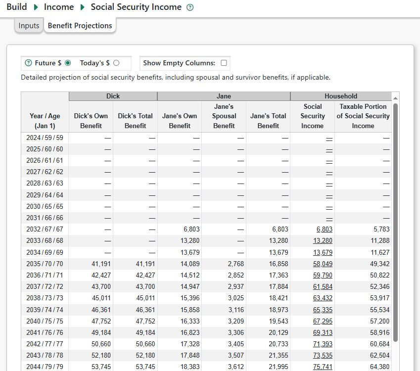
Options for Defining the Start and Stop of Expense Streams
With the exception of Healthcare, all expense streams start and stop based on a specified year.
Personal Property
The Personal Property page is used to enter information related to property, such as homes and cars that you currently own or expect to purchase in the future. Pralana models various types of loans, operating costs and capital improvements for each property as well as capital gain or loss when properties are sold.
Personal Property Step-Up in Basis on Death of First Spouse
For two-spouse plans, Pralana will apply a basis adjustment to personal property owned in the year the first spouse dies. The property is assumed to be jointly owned, and the size of the adjustment depends on your state of residence in that year:
Community property states: The property receives a 100% step-up in basis. All unrealized long-term capital gains are eliminated.
Common-law (non-community-property) states: Half of the unrealized LTCG are eliminated.
Pralana applies this adjustment in the year of death. If the first spouse’s year of death is before the plan starts, Pralana will assume you entered the appropriate basis as of the plan’s start and will not apply a further adjustment.
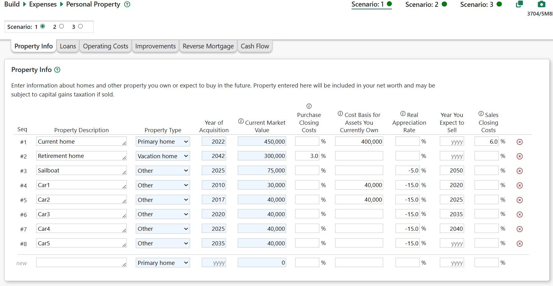
Property Info
Property Description: A brief description for each property.
Property Type: Use the pull-down menu to specify either “Primary Home”, “Vacation Home” or “Other”. This is used to determine whether the interest paid is tax deductible and whether some or all associated capital gains can be excluded from your income when the asset is sold. If you select either “Primary Home” or “Vacation Home”, Pralana will assume the interest paid is tax deductible.
Year of Acquisition: For assets you currently own, enter the year they were acquired. For assets you plan to buy in the future, enter the year you plan to make the purchase.
Current Market Value: Enter the current market value for assets you currently own as well as those you plan to buy in the future. For the latter, this will be the basis cost used in capital gains calculations. See the ‘Improvements’ section below for notes about improvements made in the past.
Purchase Closing Costs: For future purchases, enter the percentage of the purchase price that will be added as an expense in the year of purchase. Do not include the loan origination fee, which is entered on the loan page. This field is ignored for past purchases.
Cost Basis for Assets You Currently Own: This applies only to properties you already own and is the price you paid or the property’s value at the time you acquired it. This will be used by Pralana in computing capital gains. See the ‘Improvements’ section below for notes about improvements made in the past.
Real Appreciation Rate: This rate is relative to the inflation rate you specified on the Build > Get Started > Scenario Assumptions > Inflation page. Therefore, just leave this blank if you expect this asset to appreciate at the rate of inflation. Enter a negative number if you expect the asset to depreciate over time, such as most cars and boats. For Homes only, the Market Value will escalate at this rate from the Starting Year forward. All other property types will escalate in price at the inflation rate until they are purchased. Thereafter, they will appreciate or depreciate based on the rate specified here.
Year You Expect to Sell: By specifying a sale date, Pralana will terminate all expenses associated with this property on that date. You can leave this field blank if you do not plan to sell the property.
Sales Closing Costs: Enter a percentage of the sales price that will come out of your equity at the time this asset is sold. This can include sales commissions and other closing costs.
Loans
Pralana supports four types of loans on personal property: Purchase loans (first mortgages), Refinance loans (which may include cash out), Home Equity Loans and Home Equity Lines of Credit (HELOCs). For HELOC’s you may define the year(s) and amount(s) of draws. Additionally, there is a Loan Amortization tab where you can see loan annual amortization schedules.
Loan input fields vary depending on the type of loan and whether the loan was originated prior to the plan start year (existing loans) or in/after the plan start year (future loans). Fields with a blue background are required. Fields that are informational or not applicable will be greyed out and not editable.
Common Loan Fields
The various loan types may have these input fields. See additional information below for fields applicable to certain loan types.
Property: Select one of the properties defined on the Property Info tab.
Origination Year: Enter the loan’s origination year. For purchase loans, the origination year is assumed to the year the property was purchased and is not editable.
Interest Rate: Enter the annual interest rate of existing loans. (Pralana only supports fixed rate loans.)
Term: Enter the loan’s term in years. This is optional for loans originated in the past (unless the loan has an interest only period) because Pralana will calculate the amortization using the Interest Rate, Balance at Plan Start, and Monthly Payment.
Balance at Plan Start: For existing loans enter the outstanding loan balance as of the plan start date. This field is disabled for future loans.
Monthly Payment: For existing loans, enter the loan’s monthly principal and interest payment. Do not include any escrow amounts for taxes/insurance or extra principal payments you intend to make.
Loan Amount: For future loans, enter the anticipated loan amount in today’s dollars. The difference between the purchase price and this loan amount will be your downpayment. You may separately define a piggyback home equity loan.
Origination Fee: For future loans, enter assumed loan origination fees as a percentage of the loan amount.
% Tax Deductible: Enter the percentage of the loan interest that is deductible. The default value is 100% for homes and 0% for other types if property.
Notes: Enter a description or other notes about the loan (up to 255 characters).
Optional Loan Fields
All loans have these optional fields which are less commonly used. Click the Show Optional Fields checkbox to reveal these fields.
Interest-Only Period: You may specify an interest-only period, in years. The interest only period starts in the origination year. During the interest-only period, Pralana will calculate and apply the interest-only payment and the loan’s principal balance will remain unchanged (unless you also specify an additional principal payment). After the interest only period:
For existing loans, Pralana will use your entered monthly payment to amortize the loan until it is paid off.
For new loans, Pralana will calculate the monthly payment required to amortize the loan balance from the start of the repayment period until the end of the remaining loan term.
Early Pay-Off Year: If you specify an early pay-off, the loan balance (at the end of the prior year) will be paid-in-full at the start of this year. The lump-sum payoff amount will be shown on the amortization schedule and treated as a property expense in the pay-off year.
Extra Principal Payments (Annual $): You may specify additional principal payments by entering an annual amount. Pralana will apply these additional principal payments in the years specified (but not prior to plan start).
Extra Principal Payments Start: Enter the year you plan to start making the excess payments. For existing loans, Pralana assumes that any additional principal payments may in the past are reflected in the Balance at Plan Start field.
Extra Principal Payments Stop: Enter the year you plan to stop making excess payments (i.e., the last year of those payments). Leave this field blank if you intend to make the extra payments until the loan is paid-in-full.
Refinance
The loan amount field does not apply to refinance loans. If the loan was originated in the past, enter the Balance at Plan Start. If the loan is originated in the future, the loan amount will be the balance on any existing first mortgage on the property at the time of the refinance, plus any cash out amount you specify.
Cash Out % of Equity: You may specify that future refinance loans be ‘cash out’ refinance loans by entering a percentage in this field. Pralana will calculate the cash out amount based on your equity (property value minus the balance of the loan being paid off). The new loan amount will be the payoff on the old first mortgage (if any) plus the cash out amount.
Home Equity Loan
This is a 2nd mortgage loan with a fixed loan amount and monthly payment, though you may define an interest-only period. For future home equity loans, you will receive the loan proceeds, minus any origination fee, on January 1 of the origination year.
Loan Amount as % of Equity: For future home equity loans, specify the loan amount as a % of equity in the origination year. Pralana will calculate the loan dollar amount based on this percentage times your equity in the that year.
Home Equity Lines of Credit (HELOC)
You may define HELOCs on primary and vacation homes. HELOCs initially have a defined credit limit and $0 balance. HELOCs have a draw period during which you may ‘draw’ amounts on the HELOC Draws tab. During the draw period, Pralana will make monthly interest-only payments based on the balance, if any. At the end of the draw period, the repayment period begins. Pralana will calculate the monthly payment based on the balance at the start of the repayment period, interest rate, and the number of repayment years.
Draw Period: The duration of the draw period, in whole years. During this period, only interest payments will be made.
Repayment Period: The duration of the repayment period, in whole years. During this period, no draws may occur. Pralana will apply the calculated monthly payment until the loan is paid off.
Line Limit (pre-existing HELOCs): Enter the line limit for HELOCs originated in the past.
HELOC Draws
On this page you may specify HELOC draws. The data entry fields are:
Select HELOC: Select a HELOC from the dropdown list.
Origination Year: Shows the origination year for the selected HELOC. This field is informational and not editable.
Draw Period: Shows the draw period in years for the selected HELOC. This field is informational and not editable.
Draw Amount: Enter the draw amount in today’s $. Pralana will inflate the draw amount from plan start year until the draw year.
First Draw Year: Enter the year of the first draw.
# of Annual Draws: You may specify that the draw occurs for up to 10 consecutive years.
Notes: Enter a description or other notes about the draw (up to 255 characters).
Loan Amortization
On this tab, you may select a loan and see the loan cash flow and amortization schedule.
Personal Property Operating Costs
Pralana allows you to define custom operating cost categories and amounts for your properties, such as maintenance and real estate taxes.
Categories
Use this tab to define operating cost categories. These categories are available in all scenarios. Please note that you do not need to specify the following cost categories, as they are always assumed to exist: Property Taxes, Change in Property Tax Rates After Age 65, and Insurance. When you go to the Operating Costs tab, it will be pre-populated with the categories defined on this tab.
You may optionally enter a positive or negative inflation adjustment. Operating costs will be inflated using your general inflation rate, plus the adjustment you specify.
Amounts
Use this page to enter the annual expenses for each of your properties. The amounts are scenario specific. Each of the properties you have defined on the Property Info tab will appear as rows in this table and the expense categories you have defined on the Operating Cost Categories tab will appear as columns in this table. When Pralana does its projections, these expenses will only be included in your expense profile during the period in which you own the associated property.
Actual or Expected Property Taxes: This MAY be included in your monthly payments to the loan company which holds it in escrow until the taxes are due. Regardless, they should be separated from principal and interest in this table because they are affected differently by inflation and are always deductible if you itemize.
Change in Property Tax Rates After Age 65: Pralana allows you to specify a separate inflation rate for your property taxes after reaching age 65. The intent here is to allow you to model a freeze or a partial freeze of your property taxes when you reach age 65. This rate is relative to the inflation rate you specified on the Build > Get Started > Scenario Assumptions > Inflation page. So, if your taxes are frozen and general inflation is 3%, enter a -3% here. Just leave this blank if you expect your property taxes to increase at the rate of inflation.
Actual or Expected Insurance: Like property taxes, this MAY be included in your monthly payments to the loan company which holds it in escrow until the insurance premium is due. Regardless, this should be separated from principal and interest in this table because it is affected differently by inflation and is not tax deductible.
Operating & Maintenance Costs: This column of the table is highlighted with a gray background because the values are calculated by Pralana and are write-protected. They are simply the sum of the values entered in the columns which appear to the right.
Category-by-category Expenses: This is where you enter the annual amount in today’s dollars for each of the cost categories you specified on the Cost Categories tab.
Projections
This tab shows your inflated operating costs during the scenario years in which you own the property.
Improvements
On this tab, you can specify capital improvements you plan to make to a home in the future. Select the property and enter the year and cost of the improvement, in today’s dollars. Each improvement will become an expense in the associated year and will increase the value of the property by the same amount.
For improvements made in the past, you may enter them on either the:
Improvements tab: Pralana will inflate the amount you enter and add it to the property’s value as the value changes with inflation over the years. Pralana will also back-into the original cost at the time of the improvement and add that amount to the property’s cost basis.
Property Info tab: You may include the value added by the improvement in the amount you enter for the ‘Current Market Value’. You will need to separately include the original cost of the improvement, in the year it was made, in the amount you enter in the ‘Cost Basis for Assets You Currently Own’ field.
Do not include the improvement cost and value on both tabs, to avoid double-counting.
Reverse Mortgage
Pralana supports a reverse mortgage on your Primary Home as specified on the Property Info page and the details of this mortgage are specified on this tab. The projection of the reverse mortgage, including the annual income stream, the balance of the mortgage and the accrued interest can be found on the Review > Tabular Projection > Reverse Mortgage page. The outstanding mortgage balance will become an expense if the associated property is sold during the modeling period and the accrued interest in the final year will be included in the itemized deductions for the sale year. Reverse mortgage balance will be included as a negative value in calculating your net worth. In actual practice, reverse mortgages cannot “go upside down”, where the mortgage balance exceeds the value of the home; however, Pralana does not implement this restriction and it is therefore possible for you to set up the case where the reverse mortgage balance exceeds the value of the home.
Inputs
Property Description: Use this pull-down menu to select from the list of properties defined on the Property Expenses page.
First Year: This defines the year the reverse mortgage began or is to begin. You can enter a year in the past for reverse mortgages already in effect at the start of the modeling period.
Principal Amount: This is the current balance on a reverse mortgage established prior to the start of the modeling period. Leave blank if your loan is to be established in the future.
APR: This is the annual percentage rate you will be paying on the mortgage.
Initial Fees: This is the initial fee to be paid when the mortgage is established, as a percentage of the value of the associated property.
Annual Fees: This is the annual fee as a percentage of the outstanding balance of the reverse mortgage.
Pay-out Option, with the choices being:
Lump sum
Tenure (which is paid for the life of the mortgage)
Term (which is paid for a specified number of years)
Annual Pay-out Amount: This is the annual dollar amount of the income stream to be paid by this reverse mortgage.
Term: This is the duration (in years) of the pay-out and it is only applicable if a pay-out option of “term” is selected.
Cash Flow Projection
This tab shows the cash flow and related metrics for the reverse mortgage.
Cash Flow
Cash Flow Summary
On this tab, you will find a summary spanning all your properties with the following data: expenses, loans, valuation, purchase details, sale details, equity loans, and tax information. Click on underlined amounts for the pop-up Metric MRI showing supporting details for that metric.
Cash Flow by Property
On this tab, you will find the information presented on the Cash Flow Summary tab broken down by property. Click on underlined amounts for the pop-up Metric MRI showing supporting details for that metric.
Rental Property
The Rental Property page is used to enter information related to rental properties that you currently own or expect to purchase in the future. Pralana models rental income, operating costs, capital improvements and various types of loans for each property. It calculates operating income, passive activity loss limitations, depreciation, and capital gains/losses using these Federal tax forms:
Schedule E: Supplemental Income and Loss
Form 8582 Passive Activity Loss Limitations
Form 4797 Sales of Business Property
Rental Property Step-Up in Basis on Death of First Spouse
For two-spouse plans, Pralana will apply a basis adjustment to rental property owned in the year the first spouse dies. The property is assumed to be jointly owned, and the size of the adjustment depends on your state of residence in that year:
Community property states: The property receives a 100% step-up in basis. All unrealized long-term capital gains are eliminated.
Common-law (non-community-property) states: Half of the unrealized LTCG are eliminated.
Pralana applies this adjustment in the year of death. If the first spouse’s year of death is before the plan starts, Pralana will assume you entered the appropriate basis as of the plan’s start and will not apply a further adjustment.
Passive Activity Losses (PALs): Pralana adjusts suspended passive activity losses when a spouse dies. In the year of death, the full PAL balance remains available on the final joint return. Beginning in the following year, Pralana reduces the PALs by the deceased spouse’s share (typically 50% in non–community-property states and 100% in community-property states), and only the survivor’s portion is carried forward.
Depreciation: Pralana does not currently adjust depreciation schedules when a spouse dies. In reality, a death-related step-up would require continuing the original depreciation on the survivor’s portion (in non–community-property states) and starting a new depreciation schedule for the stepped-up portion. Pralana does not perform this split and continues using the original depreciation schedule for the entire property.
Rental Property Info
Asset Description: Simply a brief description of each property
Year of Acquisition: For assets you currently own, enter the year they were acquired. For assets you plan to buy in the future, enter the year you plan to make the purchase.
Current Market Value: Enter the current market value for assets you currently own as well as those you plan to buy in the future. For the latter, this will be the basis cost used in capital gains calculations.
Purchase Closing Costs: For future purchases, enter the percentage of the purchase price that will be added as an expense in the year of purchase. Do not include the loan origination fee, which is entered on the loan page. This field is ignored for past purchases.
Cost Basis for Assets You Currently Own: This applies only to properties you already own and is the price you paid or the property’s value at the time you acquired it. This will be used by Pralana in computing capital gains.
Real Appreciation Rate: This rate is relative to the inflation rate you specified on the Build > Get Started > Scenario Assumptions > Inflation page. Therefore, just leave this blank if you expect this asset to appreciate at the rate of inflation. Enter a negative number if you expect the asset to depreciate over time, such as most cars and boats. For Homes only, the Market Value will escalate at this rate from the Starting Year forward. All other property types will escalate in price at the inflation rate until they are purchased. Thereafter, they will appreciate or depreciate based on the rate specified here.
Year You Expect to Sell: By specifying a sale date, Pralana will terminate all expenses associated with this property on that date. You can leave this field blank if you do not plan to sell the property.
Sales Closing Costs: Enter a percentage of the sales price that will come out of your equity at the time this asset is sold. This can include sales commissions and other closing costs.
Depreciation Period: Enter the number of years over which this property will be depreciated.
Improvement Percentage: This identifies the percentage of the value of the property associated with improvements rather than land. The improvements will be depreciated over the period specified in the Depreciation Period field.
Rental Income: Enter the annual rental income from the property.
Rent Inflation Rate: Enter the percentage by which the rent on the property is increased annually. Note: your general inflation rate is not applied to rental income. If your Rent Inflation Rate is blank or 0%, rental income will not increase over time.
Loans
Pralana currently supports three types of loans on rental property: Purchase loans (first mortgages), Refinance loans (which may include cash out) and Equity Loans. In the future, we may add support for Lines of Credit which would be similar to HELOCs on a primary residence. There is a Loan Amortization tab where you can see loan annual amortization schedules.
Loan input fields vary depending on the type of loan and whether the loan was originated prior to the plan start year (existing loans) or in/after the plan start year (future loans). Fields with a blue background are required. Fields that are informational or not applicable will be greyed out and not editable.
Common Loan Fields
The various loan types may have these input fields. See additional information below for fields applicable to certain loan types.
Property: Select one of the properties defined on the Property Info tab.
Origination Year: Enter the loan’s origination year. For purchase loans, the origination year is assumed to the year the property was purchased and is not editable.
Interest Rate: Enter the annual interest rate of existing loans. (Pralana only supports fixed rate loans.)
Term: Enter the loan’s term in years. This is optional for loans originated in the past (unless the loan has an interest only period) because Pralana will calculate the amortization using the Interest Rate, Balance at Plan Start, and Monthly Payment.
Balance at Plan Start: For existing loans enter the loan balance as of the plan start date. This field is disabled for future loans.
Monthly Payment: For existing loans, enter the loan’s monthly principal and interest payment. Do not include any escrow amounts for taxes/insurance or extra principal payments you intend to make.
Loan Amount: For future loans, enter the anticipated loan amount in today’s dollars. The difference between the purchase price and this loan amount will be your downpayment. You may separately define a piggyback home equity loan.
Origination Fee: For future loans, enter assumed loan origination fees as a percentage of the loan amount.
% Tax Deductible: Enter the percentage of the loan interest that is deductible. The default value is 100%.
Notes: Enter a description or other notes about the loan (up to 255 characters).
Optional Loan Fields
All loans have these optional fields which are less commonly used. Click the Show Optional Fields checkbox to reveal these fields.
Interest-Only Period: You may specify an interest-only period, in years. The interest only period starts in the origination year. During the interest-only period, Pralana will calculate and apply the interest-only payment and the loan’s principal balance will remain unchanged (unless you also specify an additional principal payment). After the interest only period:
For existing loans, Pralana will use your entered monthly payment to amortize the loan until it is paid off.
For new loans, Pralana will calculate the monthly payment required to amortize the loan balance from the start of the repayment period until the end of the remaining loan term.
Early Pay-Off Year: If you specify an early pay-off, the loan balance (at the end of the prior year) will be paid-in-full at the start of this year. The lump-sum payoff amount will be shown on the amortization schedule and treated as a property expense in the pay-off year.
Extra Principal Payments (Annual $): You may specify additional principal payments by entering an annual amount. Pralana will apply these additional principal payments in the years specified (but not prior to plan start).
Extra Principal Payments Start: Enter the year you plan to start making the excess payments. For existing loans, Pralana assumes that any additional principal payments may in the past are reflected in the Balance at Plan Start field.
Extra Principal Payments Stop: Enter the year you plan to stop making excess payments (i.e., the last year of those payments). Leave this field blank if you intend to make the extra payments until the loan is paid-in-full.
Refinance
The loan amount field does not apply to refinance loans. If the loan was originated in the past, enter the Balance at Plan Start. If the loan is originated in the future, the loan amount will be the balance on any existing first mortgage on the property at the time of the refinance, plus any cash out amount you specify.
Cash Out % of Equity: You may specify that future refinance loans be ‘cash out’ refinance loans by entering a percentage in this field. Pralana will calculate the cash out amount based on your equity (property value minus the balance of the loan being paid off). The new loan amount will be the payoff on the old first mortgage (if any) plus the cash out amount.
Equity Loan
This is a 2nd mortgage loan with a fixed loan amount and monthly payment, though you may define an interest-only period. For future equity loans, you will receive the loan proceeds, minus any origination fee, on January 1 of the origination year.
Loan Amount as % of Equity: For future equity loans, specify the loan amount as a % of equity in the origination year. Pralana will calculate the loan dollar amount based on this percentage times your equity in the that year.
Loan Amortization
On this tab, you may select a loan and see the loan cash flow and amortization schedule.
Rental Property Operating Costs
Pralana allows you to define custom operating cost categories and amounts for your properties, such as maintenance and real estate taxes.
Categories
Use this tab to define operating cost categories. These categories are available in all scenarios. You may optionally enter a positive or negative inflation adjustment. Operating costs will be inflated using your general inflation rate, plus the adjustment you specify.
Amounts
Use this tab to enter the annual operating expense amounts for each of your rental properties. The amounts are scenario-specific. Each of the properties you have defined on the Rental Property Info tab will appear as rows in this table and the expense categories you have defined on the Expense Categories tab will appear as columns in this table. If you wish to add additional columns, you need to go back to the Operating Cost Categories tab and add the additional cost categories there, and that will result in the addition of corresponding columns on the Operating Costs tab. When Pralana does its projections, these expenses will only be included in your expense profile during the period in which you own the associated property.
The column on the far left side of the page is entitled “Summary of Annual Operating Costs” and contains read-only fields which are a summation of the data you manually enter in the columns to the right for each of your properties.
Projection
This tab shows your inflated operating costs during the scenario years in which you own the property.
Improvements
This tab enables you to model improvements to your rental property. If you have made improvements in the past which are still in the depreciation period, you should enter these improvements here and *not* include the cost of the improvement in the property’s Current Market Value and Cost Basis. Pralana will apply the correct amount of depreciation for the improvement based on the improvement year, cost and depreciation period.
Year: Enter the year the improvement was or will be made.
Cost: Enter the cost of the improvement, in Today’s $. For future improvements, the cost will be inflated until the year of the improvement and will be treated as an expense in that year. The cost will also increase the property value and basis.
Depreciation Period: Specify the number of years over which this improvement will be depreciated.
Cash Flow
Cash Flow Summary
On this tab, you will find a summary spanning all your properties with the following data: valuation, expenses, income, and tax information. This includes Schedule E Income/Loss, Adjusted Basic and Depreciation. Click on underlined amounts for the pop-up Metric MRI showing supporting details for that metric.
Cash Flow Details
On this tab, you will find property valuation, expenses, income and tax information for one specific property which you can specify through the pull-down menu in the field entitled “Property”. Click on underlined amounts for the pop-up Metric MRI showing supporting details for that metric.
QBI Eligibility
Eligible for QBI Deduction?: You’ll need to check the box if the expenses on this property are eligible for the Section 199A QBI deduction. If checked, Pralana will deduct up to 20% of the net income from your rental property business (as reflected in the Schedule E income/loss column) from your taxable income.
Children
The Children Expenses page is used to enter detailed information related to raising and educating your children. This page includes child-rearing costs through high school, but its primary focus is on the costs associated with each child’s college years.
The Children page contains three tabs: Pre-College Expense Categories, Pre-College Expenses and College Expenses. Two of these tabs will contain child-unique rows for the children defined on the Build > Get Started > Demographics page. Please note that your children are specified via the Build > Get Started > Basic Plan Information page.
Pre-College Expense Categories
The table on this page enables you to specify the expense categories in which you will enter expenses on the Pre-College Expenses page, and these categories will apply to all scenarios.
Pre-College Expenses
You can use the table on this page to define child-specific costs for the time from the beginning of the modeling period to the year in which each child begins college, and these costs can be scenario-specific. The table will contain one row for each of your dependent children and one column for each of the expense categories defined on the Pre-College Expense Categories tab.
College Expenses
Use this page page to define child-specific college costs for each scenario. Pralana allows you to specify overall costs for college and the percentage of that cost you plan to pay. It then allows you to specify whether those costs will be paid as they are incurred, by student loans or by the 529 account. If a 529 account is chosen, Pralana will calculate the annual contributions required, if applicable.
College Start Year: Enter the year the child will begin college. Alternatively, enter the high school graduation year (or the last year you plan to provide support) for dependent children not planning to attend college.
Annual College Costs (Today’s $): Enter the entire annual cost, based on your research at collegeboard.com or elsewhere. Include all costs unique to this child and do not duplicate on the Other Expenses tab. For dependent children not attending college, enter your annual cost of supporting them. Pralana assumes you will include all costs associated with your support for this child in this field, which is separate and independent from the costs captured in the worksheet below this table which are unique to the period prior to the child starting college.
# of Years in College: Enter the number of years you expect each child to be in college, in whole years. For dependent children not planning to attend college, enter the number of years you will be providing support after high school graduation. If none, just leave blank.
% of the Cost You Plan to Fund: Enter the % of the cost you expect to cover (use this option if you are expecting the child to bear some of the cost or to get a scholarship, etc.).
How Do You Intend to Fund Each Education? Pralana allows you to model the funding of college expenses in one of three ways:
Pay as you go: Annual college costs will treated as expenses in the years the child is in college
529 Plan: Pralana will calculate annual 529 contributions cover the college expense, if the initial 529 Plan balance (from the Initial Balances page) and annual growth is not sufficient to cover the expenses. These contributions will start in your plan start year and continue until all college expenses funded by the 529 plan have ended (last child finishes college). Pralana assumes that 100% of college costs are qualified costs. Your contributions to a 529 Plan are treated as expenses in the year they are paid and are shown on the Review > Tabular Projections > Expenses > Expense Details > Children page. Interest earned on the account is not included in your taxable income.
Student loan: Pralana will model a loan beginning in the year the child begins college for the total amount of the college education that you are paying, for the duration and interest rate you specify.
Calculated Values
Based on your inputs, Pralana will calculate the following amounts for each child and in total:* Total College Cost (Future$)*: This is the sum of the projected (inflated) total cost of college (amounts paid to the school) during your plan years in future $, regardless of who is paying the cost or how it is paid. Your cost may be lower (if funded by the 529 account due to annual growth) or higher (if funded by a student loan with interest).
Your Share of the Cost (Future$): This is the sum of your share of the total college cost, regardless of how you pay it. The actual amount you pay may be:
Lower if college expenses are paid from a 529 account. The 529 account will likely have annual growth/appreciation to help offset some of the costs.
Higher if costs are funded by a student loan. Total loan payments will be your share of the college cost plus interest on the loan.
Your Total 529 Plan Contributions: If you specify that your share of college costs will be funded by the 529 account, Pralana will calculate the annual contributions needed. These contributions begin in the first year of your plan and factor in your initial 529 plan balance, the college cost and timing, and annual growth in the 529 plan. Note: Pralana does not currently factor in any Scheduled Withdrawals (Transfers) into or out of the 529 account when calculating the annual contributions.
Your Estimated College Expense: This is the sum of the expense you incur for college costs, in future $, during the plan. Your expense may be lower or higher than the amount paid to the college because:
If college costs are paid from a 529 account, your expense will be the required 529 contributions calculated by Pralana.
Growth in the 529 account will offset some of the college cost.
Contributions you made to the 529 plan prior to the plan start are not included since these amounts pre-date your plan.
Any 529 account initial balance will be factored into the annual contribution calculation.
*Any Scheduled Withdrawals you may define from another account into the 529 account are not factored into Pralana’s calculated 529 contributions.
If college costs are paid by a student loan, your expense will be the sum of the loan payments which likely include interest.
Student Loan Amortization
If you have specified that the college expenses for one or more children are to be covered via a student loan, this page will show you the amortization of those loans on a child-by-child basis. Just select the desired child via the pull-down menu and the page will be populated with the corresponding details.
Healthcare / Long-Term Care
Healthcare costs can vary dramatically as you transition from your working years to your retirement years and then again following the death of a spouse. This page is designed to capture those changing annual costs in today’s dollars while allowing you to specify which of those costs are to be paid with pre-tax dollars.
General Healthcare Settings
By default, Pralana assumes that you will begin Medicare at age 65. If at/after age 65 you are covered by an employer’s health plan, you may want to delay enrolling in Medicare.
Your Medicare Start Age, Year, Date or ‘R’: Use this field to specify that you will enroll in Medicare after you turn 65.
Spouse Medicare Start Age, Year, Date or ‘R’: Use this field to specify that your spouse (if married) will enroll in Medicare after age 65.
% Reduction in Healthcare Expenses for Survivor: Your healthcare expenses will likely decrease upon the death of one marriage partner, so Pralana allows you to specify that reduction as a percentage of the expenses you have identified above; however, this will not affect automatically calculated Medicare premiums because those are calculated on a per-person basis. Enter the expected reduction in healthcare expenses after the first spouse dies. (0% or blank = no reduction, 100% = the expenses will be $0).
Medicare Settings
The section at the top of the Healthcare Expenses page has inputs related to calculation of Medicare Part B premiums and surcharges and Part D surcharges.
IRMAA stands for “Income-Related Monthly Adjustment Amount” which is a per-person surcharge added to the base Medicare monthly premium amount based on your Medicare MAGI, defined below. There are several income-based tiers of surcharges, with higher income individuals paying higher surcharges. The first tier has no surcharge. For 2025, for example, households filing as Married Filing Jointly and having Medicare MAGI at or below $212,000 have no surcharge. Between $212,001 and $266,000 the IRMAA (surcharge) is $74 for Part B and $13.70 for Part D. The income limits for each tier are inflated annually. Pralana shows you the IRMAA income tiers and amounts at Review > Tax Forms & Brackets > Tax Brackets.
Medicare MAGI is your modified adjusted gross income (MAGI) used to calculate IRMAA. For any year, your MAGI is your Federal Adjusted Gross Income (AGI) from the 2nd prior year plus any tax-exempt interest in that 2nd prior year.
By default, Pralana will calculate Medicare Part B premiums and surcharges (IRMAA) and Part D IRMMA (but not premiums) based on Medicare MAGI in the 2nd prior year. Pralana uses published Medicare Part B premiums and IRMAA surcharges based on your Medicare modified adjusted gross income (MAGI) for the 2nd prior year. Medicare Part B premiums and IRMAA brackets are adjusted annually based on your general inflation rate plus inflation adjustments for Medicare premiums and IRMAA income limits, if any, you define on the Scenario Assumptions > Inflation page.
Part D Premiums: Because you may select from many different Part D drug plans, Pralana cannot auto-calculate your Part D premium. Instead, include any Part D premium in the Healthcare Expenses section below.
Tip: If Pralana is calculating your Medicare premiums, you can see your Medicare MAGI and Part A & Premiums at Review > Expenses > Expense Details > Healthcare page. Click on a number in the ‘Medicare MAGI’ or ‘Medicare Premiums’ columns to see the Metric MRI detailing how the amounts are calculated.
Caution: If you check the auto-calculate boxes, do not also include Basic Medicare Part B premiums and Part D surcharges in the Insurance Premiums in the Healthcare Expenses section.
If you have Medicare supplemental, advantage or other insurance premiums, you will need to enter these in the Healthcare Expenses section below.
Auto-calculate Medicare Part B premiums?: By default, Pralana will calculate Medicare Part B premiums and surcharges (IRMAA) based on Medicare MAGI in the 2nd prior year. Uncheck the boxes to disable this calculation.
Include Part D IRMAA surcharges?: By default, Pralana will calculate Medicare Part D IRMMA (but not premiums) based on Medicare MAGI in the 2nd prior year. Uncheck the boxes to disable one or disable this calculation. Some people have medical plans (e.g. military TRICARE for Life) that provide drug coverage outside of Medicare Part D and which are not subject to Part D IRMAA. Note, if “Auto-calculate Medicare Part B premiums?” is disabled, Pralana will also not calculate Part D IRMMA.
If you will be enrolled in Medicare in the first two plan years and want Pralana to calculate Medicare premiums/surcharges, you will need to enter your Medicare MAGI for the two years prior to the plan start year because of the two-year look-back. Caution: Pralana will underestimate your Medicare Part B premiums if you check the “Auto-calculate…” box but leave the MAGI fields blank and you are on Medicare in the first two years of the modeling period.
Medicare MAGI last year: Your Federal Adjusted Gross Income (AGI) from IRS Form 1040 line 11, plus tax-exempt interest from Form 1040, line 2a, for the year prior to your Pralana plan’s start year.
Medicare MAGI two years ago: Your Federal Adjusted Gross Income (AGI) from IRS Form 1040 line 11, plus tax-exempt interest from Form 1040, line 2a, for the year 2 years before your Pralana plan’s start year. For example, if your plan starts in 2026, calculate Medicare MAGI using the AGI and tax-exempt interest from your 2024 Form 1040.
Medicare MAGI Overrides
Normally, Medicare IRMAA is calculated using your Medicare (MAGI) from two years prior, as described above. If you experience a life-changing event—such as retirement or a significant reduction in income—you may request that Medicare recalculate IRMAA using a more recent, lower income amount. This is done by filing Form SSA-44 with the Social Security Administration.
The Medicare MAGI Overrides feature allows you to model this adjustment directly in Pralana.
You should consider entering a Medicare MAGI override for years in which:
Your income drops materially compared to two years prior, and
The reduction is associated with a qualifying life-changing event recognized by Social Security (for example, work stoppage due to retirement).
Common examples include:
Retirement
Reduction in work hours
Loss of pension income
Death of a spouse
Divorce or marriage
For each year where you enter an override, Pralana will use the override Medicare MAGI you specify instead of the standard calculation (Federal AGI + tax-exempt interest from two years prior) when calculating IRMAA.
This override MAGI is also used when calculating Roth conversion amounts, if you have specified Medicare IRMAA bracket limits.
IRMAA surcharges for Medicare Parts B and D will be recalculated based on the overridden MAGI.
Inputs
Year: The year for which Medicare premiums, including IRMAA, should be calculated using the override MAGI you provide, instead of Federal AGI and tax-exempt interest from the 2nd prior year.
Override MAGI: Enter the Medicare MAGI that Social Security would use after a successful IRMAA appeal for the selected premium year. This amount replaces the default two-year lookback income used by Pralana for IRMAA calculations. Medicare MAGI generally equals your federal Adjusted Gross Income (AGI) plus tax-exempt interest.
Adjust for Inflation: If checked, Pralana will adjust the Override MAGI amount by your general inflation rate. Otherwise, the amount you enter will be used in the applicable year.
Life-Changing Event: Select the life-changing event that forms the basis for the IRMAA appeal. These choices correspond to the events recognized by Social Security on Form SSA-44. This field is provided for your reference and is not used by Pralana.
Notes: Optional notes for your own reference, such as assumptions used, filing status changes, etc.
Expenses by Period
Pralana provides a specially formatted table consisting of healthcare time periods which Pralana determines based on your (and your spouse’s, if applicable) retirement date(s) and Medicare start date(s).
Healthcare Expense Periods
To accomplish this, Pralana lays out the five time periods defined as follows and hides the ones not applicable to you based on your marital status, full retirement age, etc.:
Period 1: You are married and both you and your spouse are still working full time and probably have access to group insurance. This period is not applicable if you are single.
Period 2: You are either single, or you or your spouse, but not both, are still working full time. This period has the potential for a significant increase in the cost of healthcare premiums if you are married due to possible loss of access to group insurance. If healthcare coverage was being provided (in Period 1) by the employer of the spouse who retires first, be advised that retiree healthcare premiums tend to be much higher than those for active employees and this gives you the mechanism to specify those increased costs.
Period 3: You are married and both you and your spouse are retired (see note 1 below) but neither is eligible for Medicare, or you are single and not yet eligible for Medicare. If you are married, this period could be characterized by further changes in healthcare costs relative to periods 1 and 2 because employer healthcare will be replaced by some form of retiree healthcare by this point. If you are single, you could be moving from employer benefits to retiree benefits and you can plan on higher costs.
Period 4: (see note 2 below) You are married, but only one of you is enrolled in Medicare. As you move from retiree healthcare to Medicare you’ll likely see a decrease in costs and if you and your spouse become eligible for Medicare at different times, you’ll see your costs step down when the first person enrolls in Medicare then again when the second person enrolls in Medicare. This period is not applicable if you are single.
Period 5: (see note 2 below) You and your spouse are enrolled in Medicare, or you are single and enrolled in Medicare. When you fully transition from retiree healthcare to Medicare, you will likely see your final reduction in costs.
Note 1: ‘retired’ is determined by your specified retirement date(s) on the Scenario Assumptions page, not by the end of the last employment because many people have post-retirement jobs.
Note 2: By default, Pralana assumes you enroll in Medicare at age 65. However, you can delay this or indicate that you are not eligible for Medicare on the Healthcare Settings page.
Healthcare Cost Inflation
Pralana will inflate the amounts you enter using your general inflation rate, plus any healthcare costs inflation adjustment you provide.
Inputs by Healthcare Period
Insurance premiums: This is the annual amount of your health insurance premiums. If you have specified that Pralana is to automatically calculate your Medicare Part B premiums/IRMAA and Part D IRMAA, be sure to exclude those costs from this field. If you check the box to “Assume ACA insurance if eligible” and provide the ACA second lowest cost silver premium, Pralana will calculate the ACA premium tax credit (subsidy) for marketplace insurance. Do not reduce your insurance premiums by the ACA subsidy amount. You can see how the subsidy is calculated in the Tax Forms > 8962 ACA Premium Tax Credit for the applicable years.
Out-of-pockets expenses: Enter your anticipated out-of-pocket healthcare expense. Do not include expenses you included as insurance premiums.
% insurance premiums paid with pre-tax $: Because no tax was paid on these amounts, they are excluded from Schedule A deductible healthcare expense calculations.
% out-of-pocket expenses paid with pre-tax $: Because no tax was paid on these amounts, they are excluded from Schedule A deductible healthcare expense calculations.
% considered business deduction: Your taxable self-employment income (as specified via one of the employment income streams on the Income page which is treated as net income) will be reduced by this amount and your QBI deduction will also be reduced by 20% of this amount while the TCJA of 2017 tax law remains in effect. Caution: Be sure not to double-dip here by claiming these expenses as both paid with pre-tax dollars and eligible for a business deduction.
Assume ACA insurance if eligible?: Simply check the box to indicate “yes”, and that will tell Pralana to model ACA insurance for the applicable period and to apply Premium Tax Credits (subsidies) as appropriate.
ACA Second Lowest Cost Silver Plan Premium: When you have indicated to assume ACA insurance in this period, Pralana will use this amount in conjunction with your annual insurance premium and your MAGI to determine your annual ACA subsidy.
Notes: You can use this field to capture notes to yourself about the numbers you have entered in the other healthcare expense fields.
All the costs specified in the healthcare table will be escalated over time at a rate equal to the sum of the General Inflation Rate and Real Healthcare Inflation Rate specified on the Inflation tab of the Build > Get Started > Scenario Assumptions page.
Modeling the Affordable Care Act
Pralana models the provisions of the Affordable Care Act (ACA) on the Healthcare expenses page. If your Modified Adjusted Gross Income, or MAGI (your Federal AGI + the untaxed portion of Social Security benefits + any tax-exempt interest), falls between 100% and 400% of the Federal Poverty Level (FPL) in any given year (where FPL is a function of family size), you are eligible for a Premium Tax Credit (subsidy) on your ACA health insurance plan premiums. ACA rules define your expected contribution to a benchmark insurance policy premium, and that varies from about 2% to about 10% of your MAGI. As you can see in the notional illustration below, your expected contribution is a function of your MAGI, but it is not linear. That benchmark policy is defined to be the second lowest cost Silver Plan (SLCSP) available in your geographical area. The subsidy is intended to level the playing field such that everyone pays the same for the benchmark insurance policy regardless of the area of the country in which they live. So, in practice, if the cost of the benchmark policy exceeds your expected contribution you will receive a subsidy to effectively compensate for the higher cost of insurance in your area; you will not receive a subsidy if the cost of the benchmark policy is less than your expected contribution. Therefore, the subsidy equals the cost of the benchmark policy minus your expected contribution, never to go below zero. Consequently, your actual premium is a function of your MAGI, the insurance plan you select and your subsidy, and this can also never go below zero. In other words, if your subsidy exceeds the cost of your health insurance premium (for example, if you buy a bronze plan) then you will effectively pay nothing for your insurance but neither will you receive a credit. There are numerous sources of detailed information on ACA so we will not elaborate further in this manual.
To model the ACA, Pralana contains an internal table of the inflation-adjusted Federal Poverty Level and uses it to determine the MAGI limits for eligibility. It also enables you to specify whether you plan to purchase an ACA health insurance policy and to specify the annual premium of the benchmark Silver Plan (i.e., the SLCSP) in your area:mark:. Please note that the SLCSP premium is the premium for your entire family. It then uses this information to compute your annual subsidy, when applicable, and subtracts that from your annual healthcare expenses. In doing this, Pralana also models the so-called “cliff” where the subsidy immediately drops to zero whenever your MAGI exceeds the 400% FPL number by even $1. Two caveats on that, though:
The American Recovery Act of 2021 eliminated this cliff for the years 2021 and 2022, and
The Inflation Reduction Act extends the elimination of the cliff through 2025 and that is implemented in Pralana.
You can see the MAGI and your ACA subsidies on the Review > Tabular Projections pages.
Long-Term Care and Other Healthcare Expenses
This tab enables you to specify any expected long-term care (LTC) expenses as well as other healthcare expenses which do not align with the pre-defined healthcare periods. You can specify the amount, by person, in today’s dollars as well as the start age and duration in years. For each expense, you may specify whether to apply your long-term care inflation add on, your healthcare inflation add-on, or no add-on to the general inflation rate.
A future enhancement will allow you to enter the start date as an age, year, date or ‘R’.
Pralana includes these expenses on Form 1040, Schedule A: Itemized Deductions.
Term Life Insurance
Pralana’s implementation of term life insurance is located on the Build > Expenses > Term Life Insurance page and has these features:
You can specify separate policies for you and your spouse
A fixed face value is assumed for the term of the policy and neither the death benefit nor the annual premium is adjusted for inflation
You can add multiple updates to the policy with a specified term, death benefit, and annual premium
Here is a screenshot:

Cash Value Life Insurance
Cash value life insurance is a type of insurance that includes an investment-like component that gains value over the life of the policy, can be borrowed against like a loan and is paid out upon the policy holder’s death. We will not elaborate much further on this type of insurance in this manual; however, there is a large amount of related information on the Internet, and here’s a link to one such example: https://www.policygenius.com/life-insurance/cash-value-life-insurance/. Cash value life insurance is available in a variety of forms, including whole life, variable life and universal life, and each insurance company has its own variations within these major categories. Consequently, the Pralana design does not attempt to model all possible variations of this type of insurance. Rather, it models the major features of cash value life insurance and strives to provide you with the necessary controls to enable you to approximate the desired characteristics of your specific policy or policies.
Pralana’s implementation of cash value life insurance is located on the Build > Expenses > Cash Value Life Insurance page and has these features:
A fixed face value is assumed for the life of the policy and it is not adjusted for inflation
The cash value of the policy starts with a user-specified initial value, and contributions to and growth of the cash value is modeled based on a user-specified rate of return
A fixed annual premium is assumed for the life of the policy, but once the policy is “paid up” you can use your cash value to pay that premium
The death benefit can be some combination of face value and cash value and it will be treated as non-taxable income in the year of the policyholder’s death; the policy will terminate at that point and its cash value will go to zero
A one-time withdrawal of some or all the cash value is supported (loans are not supported)
Here are two merged screenshots that illustrate the Policy Information tab where you can specify the parameters to control Pralana’s modeling of cash value life insurance policies for yourself and your spouse:
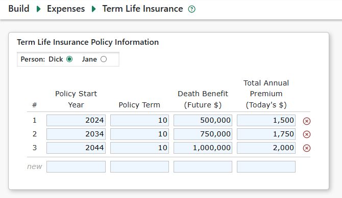
Dick has a policy established in 2024 with a face value of $100,000, an annual premium of $1178 and no cash value in the model’s starting year of 2024. As the cash value accumulates, it will have a real rate of return of 2% (and a nominal return of 5% if inflation is assumed to be 3%). 83% of the $1178 premium will be contributed to the cash value of this policy and the remaining 17% will pay for the death benefit. This policy will be considered “paid up” when the cash value builds to such a level that the annual dividend is greater than the premium, and subsequent premium payments will cease. Upon Joe’s death, this policy will pay a death benefit equal to the $100,000 face value plus 50% of the accumulated cash value. Jane plans to have a $75,000 face value policy of her own that starts in the year 2025 with an annual premium of $900. Her cash value will also have a real ROR of 2% with 83% of the premium going toward the cash value. The cash value of her policy will never be used to pay the premium and her death benefit will be the face value plus 50% of the cash value. These inputs are used to produce a projections on the Cash Value and Death Benefit Projections tab which looks like this merged screenshot:
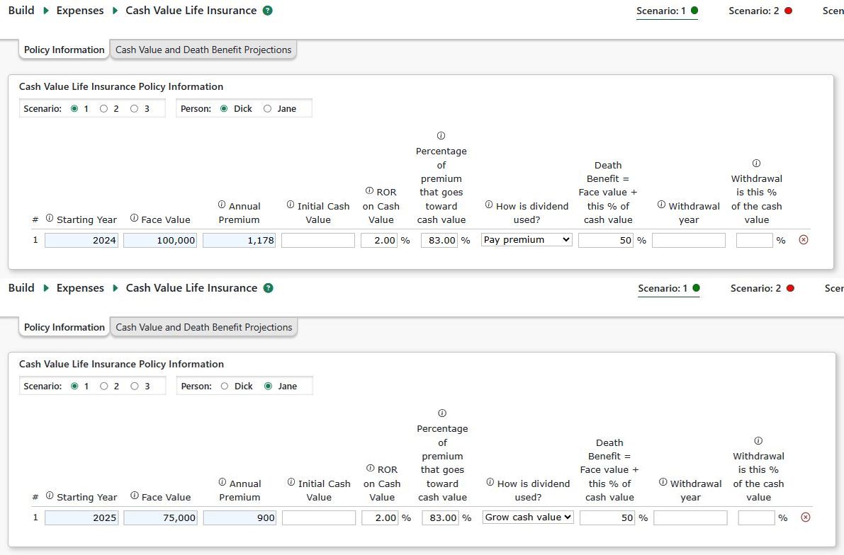
Notice that Joe’s premium ceases in 2036 when his dividend (5% of the $25,265) exceeds the $1178 premium.
Let’s now take a quick look at another example involving a withdrawal of some of the cash value.
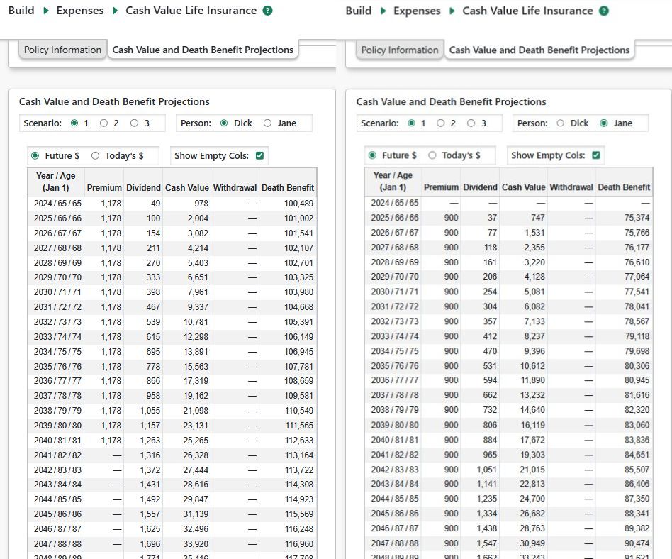
In this case, Dick plans to withdraw 50% of his cash value in the year 2042. You can see the withdrawal occur in 2042 which then causes the premium payments to resume for several years because of the associated drop in cash value and dividends. When the cash value is built back up, the premium payments are again covered by dividends.
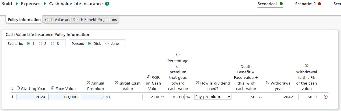
When the withdrawal occurs, those funds are deposited into the cash account. If that causes the ceiling value to be exceeded, then the excess funds will be withdrawn from the cash account and deposited into the regular savings account.
Charitable Contributions
Pralana allows you to define, for each scenario, up to 10 charitable contributions, each of which may span multiple years. These may be regular, tax-deductible charitable contributions as well as Qualified Charitable Distributions (QCDs) from a tax-deferred account.
Regular charitable contributions (non-QCDs) will be included in your annual expenses and in your Schedule A itemized deductions. Note: regular charitable contributions are considered ‘non-essential’ expenses and, after retirement, may be replaced by variable spending when using one of several Spending Strategies.
QCDs are deducted directly from the source tax-deferred account, are not taxable, and are not included in your annual expenses. Pralana assumes that QCDs will satisfy some or all of your RMDs. will be reduced by an amount equivalent to the QCD. You may define QCDs from a tax-deferred account (IRA) or an inherited traditional IRA.
For two-person plans, after the first spouse dies Pralana assumes the surviving spouse is the beneficiary of the deceased person’s tax-deferred accounts. QCDs will continue, as defined on this page, subject to the Federal limit the surviving spouse’s total QCDs from all accounts.
There are three cases where some or all of the annual QCDs amounts will be reclassified as regular charitable donations:
In years before the year the account owner reaches age 70 ½.
Anytime the source tax-deferred account has an insufficient balance to fund the QCD.
Anytime the total annual QCDs for a person (from all tax-deferred accounts) exceed the Federal limit ($108,000 in 2025).
Inputs
The table on the Build > Expenses > Charity Inputs page allows you to define charitable contributions for each scenario.
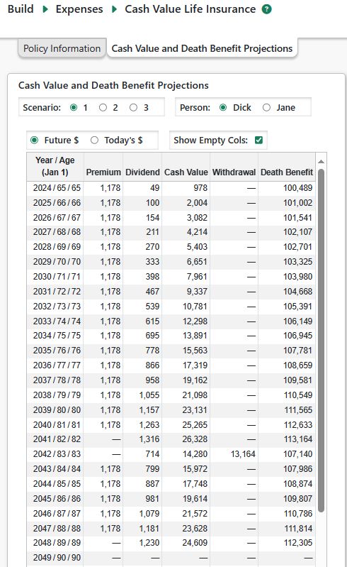
Description: A short description of the contribution.
Amount: The annual amount of the contribution in today’s $.
First Year: The year (e.g. 2030) that the contribution will start.
Last Year: The last year of the contribution. If you leave this field blank, Pralana will assume the contribution will continue until the scenario ends. For one-time contributions, make the Last Year the same as the First Year.
Is Amount Adjusted for Inflation?: If checked, Pralana will increase the amount annually using your general inflation rate.
QCD?: If checked, Pralana will treat the contribution as a Qualified Charitable Contribution.
QCD Source: For QCDs, select the source tax-deferred account. This field is ignored for non-QCD contributions.
Pralana’s tabular projections accurately reflect the treatment of your donations as QCDs or regular charitable donations based on the conditions above rather than the way they are specified on the Charity input page.
Projected Totals by Year
This tabular projection show the calculated contributions for each person and in total. It also shows the projected Federal per person limit on QCDs and any QCD amount reclassified to a regular charitable contribution.
Phased Expenses
The Build > Expenses > Phased page enables you to define, by scenario, ‘phased’ expenses. These are expenses that continue for a multi-year phase of your life.
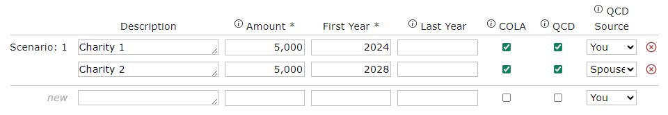
Time Periods
Use this page to define up to five time periods in which your expenses are fixed except for annual inflation adjustments. These periods are scenario-specific and could correspond to your pre-retirement years, early retirement years and late retirement years, or to any other periods/phases which you believe are likely to have substantially unique expense levels.
Categories
You can create up to 25 categories of phased expenses such as groceries, eating out, cell phones, and gifts. These categories are shared across all scenarios.
Each category may be defined as ‘essential’ or ‘non-essential’. When using most of Pralana’s variable spending strategies, essential phased expenses will continue as you defined them. Non-essential phased expenses will be replaced, after retirement, by the variable spending amount calculated for that spending strategy. Please read the section on Variable Spending Strategies for more information.
You may optionally enter a positive or negative inflation adjustment. Phased expenses will be inflated using your general inflation rate, plus any adjustment you specify for the category.
Phased Expenses % Reduction for Survivor
For plan with two spouses, you may specify a percentage by which Phased expenses will be reduced after the first spouse dies.
Amounts
For each of the time periods specified on the Time Periods tab and each of the expense categories defined on the Categories tab, you can specify the expense amount in today’s dollars. These expenses will be inflated using your general inflation rate (entered on the Build > Get Started > Scenario Assumptions page), plus any inflation adjustment you defined for the category.
Caution: Be sure not to duplicate any expenses you have already entered on the Property or Children pages. All expenses entered on this page will be escalated over time at the General Inflation Rate entered on the Build > Get Started > Scenario Assumptions page.
Projections
This tab displays a year-by-year projection of your Phased Expenses in either future or today’s dollars. It shows the totals as well as your defined categories.
Miscellaneous Expenses
The Build > Expenses > Miscellaneous page enables you to identify one-time or specific-duration expenses for each of the three scenarios. For each of these expenses, you can enter a brief description, the first year and last year of the expense, the amount in today’s dollars, whether the amount is to be adjusted for inflation (using your general inflation rate), an additional inflation adjustment/add-on (which may be positive or negative), and whether the expense is tax-deductible or is to be considered an adjustment to income. If the last year is left blank, Pralana will assume the expense continues indefinitely. For one-time expenses, the first and last years should be set to the same year.
As with Phased Expenses, line items on this page can be identified as either essential or non-essential. This enables Pralana to model variable spending in your retirement years, wherein non-essential spending is dynamically adjusted year by year as a function of the performance of your portfolio. You can read more about this in the section on Variable Spending Strategies.
Projected Totals by Year
This tab displays a year-by-year projection of your Miscellaneous Expenses in either future or today’s dollars.
Modeling Your Accounts
Pralana models the following 11 types of accounts (8 for single-person plans):
Cash account (for cash-equivalent accounts like checking and savings)
Taxable investment account
Tax-deferred accounts (for traditional IRAs and 401Ks, etc.) for you and (if married) your spouse
Roth
inherited traditional and Roth IRA accounts for you and (if married) your spouse
Health Savings Account (HSA)
529 College Savings Plan
Pralana projects future balances for each account based on the initial balance, annual growth, as well as contributions and withdrawals.
Annual growth is calculated based on the account balance and your chosen portfolio modeling method:
Simple Portfolio Modeling: Account rates of return
Advanced Portfolio Modeling: Asset rates of return and the asset allocation for each account.
The Cash Account is Central to Cash Flow Modeling
The Cash account is central to all cash flow in Pralana. All spendable income and other positive cash flows are treated as deposits to the cash account. Expenses, taxes and other negative cash flows are treated as withdrawals from the cash account. Net cash flow is the sum of the positive and negative cash flows. See Pralana’s Cash Flow Statement which shows how the net cash flow, and Cash account balance, is calculated each year.
You may specify a ‘floor’ and ‘ceiling’ for the Cash account balance on the Build > Financial Assets > Management > Cash Floor & Ceiling page.
Cash ‘overage’: If a positive net cash flow causes the Cash account’s year-end balance to exceed the ceiling, a cash ‘overage’ occurs and the excess amount is automatically transferred from the cash account to the Taxable Investment Account where that cash held in the Cash asset (even if the account has no allocation to Cash) and is not invested until the start of the next year (Jan 1), when the account is rebalanced according to the new year’s asset allocation.
Holding that deposit in cash, instead of using it to purchase assets, avoids buying assets on Dec 31 that may need to be sold the very next day as part of annual rebalancing, potentially increasing unnecessary asset turnover and triggering additional realized long-term capital gains.
Cash ‘shortage’: If a negative net cash flow causes the Cash account’s year-end balance to fall below the floor, Pralana will transfer funds into the Cash account from other accounts per your specified account Withdrawal Priority (see Build > Financial Assets > Management > Account Withdrawal Priority).
If all other accounts are depleted, Pralana will allow the Cash account balance to fall below the floor level.
If the Cash account balance falls below $0, the scenario is considered insolvent. Pralana will not force the sale of personal or rental property, or ‘call’ in any outstanding personal loans to raise cash.
NOTE: The Withdrawal Priority is not used if the Cash account’s balance never falls below the floor.
Taxable Investment Account Step-Up in Basis on Death of First Spouse
For two-spouse plans, Pralana will apply a basis adjustment in the taxable investment account in the year the first spouse dies. The account is assumed to be jointly owned, and the size of the adjustment depends on your state of residence in that year:
Community property states: The account receives a 100% step-up in basis. All unrealized long-term capital gains are eliminated.
Common-law (non-community-property) states: Half of the unrealized LTCG are eliminated.
Pralana applies this adjustment in the year of death. Any capital loss carry-overs are similarly reduced, but in the year following the spouse’s death.
Note: If the first spouse’s year of death is before the plan starts, Pralana will assume you entered the appropriate initial unrealized LTCG and capital loss carryover and will not apply a further adjustment.
Account Initial Balances
Enter the initial balances for each account type, as applicable, using the tabbed sections on the Build > Financial Assets > Account Initial Balances page. For each account type you may specify several individual accounts. Pralana models them as one and will sum the initial balances and other inputs for each type of account. It does not to model your individual accounts.
For plans with marital status ‘Married’, all accounts are treated as joint accounts except for the various tax-deferred and inherited IRA accounts.
For newly created plans, Pralana provides some default initial balances which you should change.
Henceforth, the term “account” or “accounts” refers to Pralana’s 11 account types.
As you enter/edit initial balances, Pralana shows the total initial balance across all account types in the page header, as shown in the screenshot below:
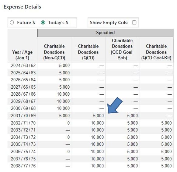
Cash Account
Enter the balances for your checking, savings and other cash-equivalent accounts. As noted previously, Pralana will aggregate these into a single virtual Cash account for which you will enter the aggregate rate of return you expect to earn on your cash holdings.
If you use Advanced Portfolio Modeling, you may also allocate a Cash asset class to other types of accounts, as well.
Taxable Investment Account
For the Taxable Investment account, the Account Initial Balances page asks for two other pieces of information to enable accurate modeling of taxation.
Unrealized Capital Gains as of the start of the modeling period: This is the account balance minus the account’s cost basis and indicates the amount of untaxed growth in the account.
Capital Loss Carryover: Losses you may have experienced prior to the model’s starting year that were not fully tax-deductible due to the annual $3000 limit on capital losses.
Contributions may be made to the Taxable Investment account in one of two ways:
Cash account ‘overages’, describe above.
Scheduled transfers from another account into Taxable Investment account.
You may specify whether interest and dividends are reinvested or transferred to the Cash account each year.
Tax-Deferred Accounts
On the Account Initial Balances page, for tax-deferred accounts you may enter the portion of the account balance that is associated with any after-tax contributions. This amount is often referred to as the account’s ‘basis’. Starting with the initial after-tax balance entered here, Pralana will model the after-tax balance going forward and proportionately include an after-tax component with pre-tax Roth conversions, required minimum distributions, and most other withdrawals.
You can contribute to tax-deferred accounts in these ways:
User-specified contributions in conjunction with employment income.
Pension rollovers as specified in conjunction with pension income.
Scheduled withdrawals/transfers from other accounts to a tax-deferred account.
Withdrawals from tax-deferred accounts may be made in the following ways:
Required Minimum Distributions (RMDs), which are calculated automatically.
Scheduled withdrawals. If defined, these will satisfy some or all of the RMD in the applicable years.
Purchase of an annuity.
Roth Conversions which you manage on the Analyze > Roth Conversions page.
Unscheduled withdrawals to cover a cash shortage. These will be in addition to RMDs in the applicable years (because RMDs were already calculated and applied).
Important note about after-tax contributions
If all of the following are true for you (or your spouse):
You have traditional IRA(s), and
You have employer-sponsored tax-deferred account(s), and
One or more of these accounts have after-tax contributions
Then Pralana will incorrectly prorate after-tax amounts for RMDs and Roth conversions. Under IRS rules:
RMDs must be prorated separately for IRAs and for each employer-sponsored plan.
Roth conversions are prorated only across traditional IRA balances and basis, and do not include employer-sponsored plan balances.
Pralana currently prorates after-tax amounts across all tax-deferred accounts combined, which can produce incorrect results in the situation described above. We may implement separate proration of after-tax amounts in a future release.
Roth Accounts
While contributions to Roth accounts are generally made with after-tax funds, account growth and withdrawals are usually tax-free. The IRS has somewhat complex rules about taxes and penalties on Roth account withdrawals that occur within 5 years of the account opening which Pralana does not implement.
You can contribute to Roth accounts in these ways:
User-specified contributions in conjunction with earned income.
Pension rollovers as specified in conjunction with pension income.
Roth conversions, which move money directly from a tax-deferred account to a Roth account.
Scheduled withdrawals/transfers from other accounts to the Roth account.
Withdrawals from Roth accounts can be made in the following ways:
Scheduled withdrawals.
Purchase of an annuity.
Unscheduled withdrawals to cover a cash shortage.
Inherited IRAs
Pralana models one Inherited traditional and one Roth IRA for you and, if married, for your spouse. The inheritance timing, initial values, and distribution rules are specified on the Build > Financial Assets > Account Initial Balances > Inherited IRAs tab.
The SECURE Act (effective for deaths on or after January 1, 2020) eliminated the standard “stretch” IRA for most non-spouse beneficiaries of inherited IRAs. Under the Act, most non-spouse beneficiaries must distribute the entire inherited IRA by the end of the 10th calendar year following the account owner’s death. However:
IRAs inherited before January 1, 2020:
These generally remain subject to the older rules, which allowed lifetime withdrawals (via a “life-expectancy” method) or in some cases a 5-year full-distribution rule, depending on the circumstances. You may specify that the distribution period is ‘Lifetime’.
IRAs inherited on/after January 1, 2020:
If the original owner of a traditional IRA had already begun taking RMDs at the time of death, the beneficiary is subject to the 10-year rule and must take annual RMDs in years 1–9. The amount must be, at a minimum, based on the beneficiary’s life expectancy in the year following the owner’s death.
If the original owner of a traditional IRA had not already begun RMDs, you must withdraw 100% of the funds by December 31 of the 10th year after the year of death. You are not required to take annual RMDs and thus may wait until the 10th year to withdraw the entire balance.
Inherited Roth IRAs: Regardless of the original owner’s age at death, these generally follow the rules for owners of traditional IRAs who had not begun RMDs (see above). Therefore, no annual RMDs are required in years 1–9, though the 10-year full distribution rule still applies.
To satisfy both requirements and provide maximum flexibility, Pralana allows you to specify the year in which you will start taking RMDs as well as the distribution period. Pralana will calculate the RMD amount by dividing the prior year’s ending balance by the number of years remaining in the user-specified distribution period. (It will not use the “life expectancy” method). The remaining balance is fully distributed in the final distribution year.
Example: If you specify a 10-year distribution period, Pralana will distribute 1/10th of the account balance in the first year, 1/9th in the second year, and so on, until the final year where 100% of the remaining balance is distributed.
Certain beneficiaries — known as “eligible designated beneficiaries” (spouses; minor children; disabled or chronically ill individuals; beneficiaries no more than 10 years younger than the decedent) — retain more flexible payout options and may still use life-expectancy-based distributions instead of being forced into the 10-year clean-out. Pralana assumes you are not an “eligible designated beneficiary” for the inherited IRAs.
Inputs
Amount: If the account was inherited prior to the starting year, this is the balance of that account on January 1 of the model’s starting year. Otherwise, it is the amount you expect to inherit in future year dollars (i.e., if you expect to inherit $50,000 in the year 2040, just enter 50,000).
Year of Inheritance: If the inheritance occurred prior to the model’s starting year, you can enter that year and Pralana will model RMDs according to that year. If you leave it blank, Pralana will assume the inheritance occurred in the year prior to the start of the modeling period. For future inheritances, just enter the year the inheritance is expected to occur (i.e., if you expect to inherit $50,000 in the year 2040, just enter 2040).
Distribution Period: Select the applicable distribution period from the drop-down list. Pralana will assume “Lifetime” if you leave this field blank. Pralana does not enforce IRS rules regarding distribution periods, so it is up to you to enter the correct period.
RMD Start Year: The IRS allows you to delay the distribution of inherited IRAs for up to 10 years in some cases, so this field (in combination with the Distribution Period field) enables you to delay the distribution until some specified year in the future.
Contributions to inherited IRAs: Per Federal law, Pralana does not permit deposits to an inherited IRA beyond the amount inherited.
Withdrawals from inherited IRAs can be made in the following ways:
Traditional inherited IRAs only: Required Minimum Distributions (RMDs), which are calculated automatically.
Scheduled withdrawals. If defined, these will satisfy some or all of the RMD in the applicable years.
Unscheduled withdrawals to cover a cash shortage. These will be in addition to RMDs in the applicable years (because RMDs were already calculated and applied).
Health Savings Accounts
Contributions to HSAs are tax deductible, account growth is tax-free, and withdrawals to pay qualified medical expenses are also tax-free (but see note below about New Jersey and California.) Withdrawals for other reasons are subject to penalties.
New Jersey and California: These states include contributions to, and annual growth in, HSAs as taxable income. Pralana assumes annual growth in an HSA is ordinary income.
The initial balance of your HSA is entered on the Build > Financial Assets > Account Initial Balances > HSA page.
In Pralana, you may specify contributions to your HSA two ways:
As employment payroll contributions made by you and/or your employer
By defining a Scheduled Withdrawal from another account into your HSA. Pralana assumes you have determined that this is a qualified contribution.
If using Simple Portfolio Modeling, you specify the annual rate of return on your HSA. If you use Advanced Portfolio Modeling, you define the asset allocation of your HSA account.
Healthcare expenses are entered on the Build > Healthcare Expenses page. If you plan to use the HSA to pay for, or reimburse yourself for, some or all healthcare expenses, then those expenses should be designated as being paid with post-tax dollars (because later they will be reimbursed with pre-tax dollars). Withdrawals are scheduled via entries in the table on the Build > Financial Assets > Scheduled Withdrawals page. Pralana maintains the HSA balance and you can see that on the Review > Tabular Projections > Accounts & Portfolios page.
529 College Savings Plans
Enter the balances of your 529 College Savings Plans, if any. Pralana will use the initial balances, along with contributions and withdrawals to project the account balance during each scenario.
Generally, annual contributions to 529 plans are made with after-tax dollars, the account funds can be invested and grow over time, and you can make withdrawals to cover qualified education expenses with no taxes on the account growth.
Contributions to the 529 Plan
If you specify that college expenses are to be paid from a 529 Plan and the plan’s initial balance plus projected growth is insufficient to cover those expenses, Pralana will automatically calculate the additional contributions required. These contributions are shown on the Review > Tabular Projections > Expenses > Expense Details > Children page.
Contributions calculated by Pralana to fund college expenses are treated as expenses in the year they are made. The amounts appear in the “529 Plan Contributions” column on the Expense Details > Children page.
Tuition Payments from the 529 Plan
Because contributions to the 529 Plan are already treated as expenses in the years they are made, withdrawals from the 529 Plan are not treated as expenses when tuition is paid.
Instead, tuition payments from the 529 Plan are shown on the Cash Flow Statement as a non-cash outflow in the “Tuition Payment from 529 Plan” column. These withdrawals are also visible on the Cash Flow > Withdrawals page.
You may specify additional funds transfers from and to the 529 account on the Scheduled Withdrawals page. Note: Scheduled Withdrawals/Transfers from/to the 529 plan are not factored into the algorithm which auto-calculates 529 contributions needed to cover college expenses.
Health Reimbursement Arrangements (HRAs)
HRAs, or Section 105 plans, provide an IRS-approved way for an employer to reimburse an employee for eligible expenses. HRAs are not explicitly modeled by Pralana. You can effectively model an HRA by simply reducing the insurance premiums and out-of-pocket expenses entered by the amount you expect to have reimbursed by your employer. You may document this calculation via the Notes fields on the healthcare expenses page.
Management
There are several important management variables that need to be specified to enable Pralana to model your accounts. Account management is controlled by the Build > Financial Assets > Management page which has seven subpages:
Cash Floor and Ceiling
Withdrawal Priority
LTCG Withdrawal Strategy
Account Fees
Deferred RMDs
Effective Tax Rate
Account Growth Settings
Cash Floor and Ceiling
As explained in the section: Account Initial Balances: Cash Account, the cash account has user-specified minimum (floor) and maximum (ceiling) balances, which are defined on this tab. The balance of the cash account will always remain in the range established by these floor and ceiling levels (unless you run out of money in all other accounts). If for whatever reason you do not wish to model a cash account, just set floor and ceiling levels to zero by entering blanks in these fields.
Key Points to Understand:
All positive net cash flows cause contributions to your cash account and all negative net cash flows cause withdrawals from your cash account.
You can specify upper and lower limits of your cash account.
Cash ‘Overage’: When the preliminary ending cash account balance exceeds the Cash Ceiling, the excess funds are transferred to your taxable investment account
Cash ‘Shortage’: When the preliminary ending cash account balance falls below the cash floor, funds are transferred in from one or more of your other accounts, in accordance with your account withdrawal priority.
Pralana’s Cash Flow Statement shows the cash inflows, outflows, net cash flow, preliminary ending cash balance, cash floor and ceiling, cash overage/shortage and the associated transferred out (when there is a cash overage) and in (when there is a cash shortage).
Account Withdrawal Priority
When a cash shortage occurs in the Cash account, Pralana will transfer funds from other accounts, in the order you specify on this page, to bring the Cash account balance back up to the ‘floor’. Starting with the top priority account, a transfer will be made to the Cash account. If the top priority account does not have sufficient balance to cover the cash shortage, Pralana will continue to make withdrawals from the 2nd and subsequent accounts until the cash shortage is covered. If all accounts become depleted, it will take the cash account below the specified floor level if necessary.
Important note: Withdrawal priority is moot if there is no negative cash flow in your plan because it only comes into play whenever you have negative cash flows that would take the cash account balance below its floor level.
To adjust the order of the accounts, simply drag and drop any account into the desired position and continue that process with the other accounts until the list is organized as you wish.
Unscheduled withdrawals: These withdrawals to cover a cash shortage are referred to as ‘unscheduled’ withdrawals because they are not defined by you or standard rules such as RMDs, etc.
Because taxes have already been calculated and included in the expenses and net cash flow, any taxable income resulting from unscheduled withdrawals is taxed in the following year. The Pralana team is working to implement an iterative tax calculation and tax income from unscheduled withdrawals in the same year the withdrawals are made by grossing up the withdrawal amount.
LTCG Withdrawal Strategy
Pralana allows you to specify whether to withdraw unrealized long-term capital gains first, last, or evenly (proportionately based on the percentage of the account or asset balance that is unrealized LTCG) when most withdrawals are made from the Taxable Investment account. If an asset is sold that has an unrealized long term capital loss, the loss will be realized proportionately.
In the Taxable Investment account, Pralana tracks balances and unrealized LTCG from year-to-year by asset class. You can see asset-level information on the Balance Sheet by clicking on an amount in the Taxable Investment column or in the Unrealized LTCG In Taxable Inv. Acct column. Then, click on the ‘Asset Details’ button.
Withdrawals from the Taxable Investment account will force a sale of assets and may trigger ‘realized’ LTCG which are taxed in the year of withdrawal (except for realized LTCG on unscheduled withdrawals which are currently taxed in the following year).
The following types of transactions result in an asset sale and may cause realized LTCG:
Account re-balancing: at the start of each year, the account is re-balanced. Over-allocated assets are sold, and under-allocated assets are purchased.
Account management fees: See details in the Account Management Fees section below.
Scheduled withdrawals and end-of-year ‘unscheduled’ withdrawals (to fund a cash shortage).
There are two types of withdrawals that never trigger realized LTCG:
Withdrawals of non-reinvested interest and dividends which are transferred to the Cash account, and
Scheduled Withdrawals from the Taxable Investment account to an External designation are assumed to be transfers of appreciated assets and do not trigger a sale. The unrealized LTCG balance is reduced by its pro-rata share of the asset or account balance.
The LTGC withdrawal strategy options are:
Distribute withdrawals evenly: LTCG will be realized in proportion to the % of asset balance that is unrealized LTCG.
Withdraw capital gains first: withdrawals will be funded by the unrealized LTCG balance (triggering realized LTCG) until depleted and then from non-appreciated assets.
Withdraw capital gains last: withdrawals will be funded by unappreciated assets (triggering no realized LTCG) until only unrealized LTCG remains.
For example, assume the Taxable Investment account has an asset with a balance of $100K of which $30K or 30% is unrealized LTCG. If a $10K scheduled or unscheduled withdrawal is made and the withdrawal strategy for unrealized LTCG is:
Evenly: $10K of the asset will be sold and withdrawn, 30% or $3K will be taxed as realized LTCG that year, the remaining balance will be $90K total / $27K unrealized LTCG.
First: $10K of the asset will be sold and withdrawn, all of which will be taxed as realized LTCG that year, the remaining balance will be $90K total / $20K unrealized LTCG.
Last: $10K of the asset will be sold and withdrawn, none of which will be taxed as realized LTCG that year, the remaining balance will be $90K total / $30K unrealized LTCG.
Account Management Fees
This page contains a simple list of your accounts where you can specify the annual management fee percentage for each of your accounts. While fees are often paid quarterly, Pralana always assumes fees are paid at the start of each year based on the balance at that time. This is a simplification and tends to be a more conservative assumption. Account assets are sold to raise funds to pay the fee and may cause realized long-term capital gains, depending on the unrealized LTCG balance and your LTCG withdrawal strategy.
Deferred RMDs
Required Minimum Distributions (RMDs) must be taken from your tax-deferred accounts when you reach the age specified by SECURE 2.0; however, if you are still employed by the company sponsoring your 401k, you can delay your RMD from that 401k until you retire. This control gives you the ability to tell Pralana that some percentage of your (and/or your spouse’s) tax-deferred account is not subject to RMDs at the age specified by SECURE 2.0. When you stop working (as specified by the retirement date milestone), Pralana will thereafter calculate RMDs based on 100% of the funds in your tax-deferred account.
Conversion Rate for Calculation of Effective Savings
You should be cautious when comparing the value of a portfolio where investments are held mostly in taxable or tax-free accounts with one where investments are held mostly in tax-deferred accounts because the funds in tax-deferred accounts are not all yours. Some of that money belongs to Uncle Sam; he just has not collected it from you, yet. To help you with this, Pralana calculates the effective buying power of your portfolio as a function of its distribution across accounts with differing taxation properties. Money held in cash, taxable and Roth accounts is counted at full value; money held in the tax-deferred accounts is derated based on the Effective Tax Rate you expect to apply to those funds when withdrawn. If you plan to leave some or all your tax-deferred accounts to your heirs, the withdrawals are likely to be different than your own tax rates. Therefore, Pralana asks you to specify the effective tax rate to be used when determining the effective buying power of those accounts, and that is done via the setting on this page.
This setting is used to create the projections on the Analyze> Scenario Analysis Comparisons and Analyze > Roth Conversion pages, where you have the option to see the results graphed in terms of absolute or effective dollars.
Account Growth Settings
The controls on the Account Growth Settings tab do two very important things within Pralana: they specify HOW the annual rate of return (ROR) for each account is to be determined and WHEN the annual ROR for each account is to be applied to model account growth. Here is a screenshot of this simple tab:
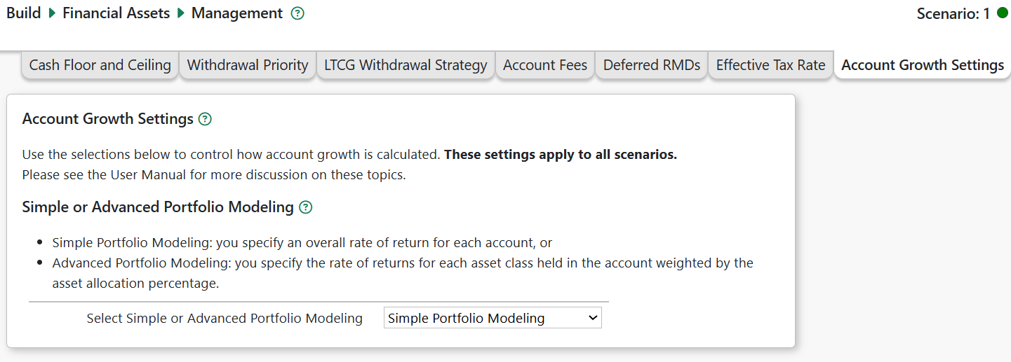
Simple or Advanced Portfolio Modeling
Pralana provides two fundamental ways of determining the ROR for each account. The simplest and most straightforward way is for you to specify it directly and the more advanced way is to derive it based on asset classes and allocations. You make your selection via the pull-down menu associated with the field called Select Simple or Advanced Portfolio Modeling. If you select Simple Portfolio Modeling, then your account RORs will be as specified on the Rates of Return tab on the Build > Financial Assets > Simple Portfolio Modeling page. If you select Advanced Portfolio Modeling, then your account RORs will be derived from your inputs on the Rates of Return and Asset Allocation/Location tabs on the Build > Financial Assets > Advanced Portfolio Modeling page. Please refer to the user manual sections corresponding to those pages for more information on this subject.
Account Growth Timing
As of October 2025, Pralana calculates account growth using each account’s asset balances, after start-of-year rebalancing and after any account management fees are deducted.
In the future, Pralana may offer the option to calculate account growth using an estimated mid-year balance. This balance will be based on the year’s starting asset balances (after rebalancing) and half of the expected credits and debits for the year.
Modeling Your Portfolio
Your portfolio is the collection of all the investments (asset classes) you hold, in all accounts. Pralana allows you to model your portfolio in one of two ways as specified on the Simple or Advanced Portfolio Modeling tab of the Build > Financial Assets > Management page:
Simple portfolio modeling: you specify the expected overall rate of return (ROR) for each account, or
Advanced portfolio modeling: you define your asset classes, their rates of return and growth taxation. Then you allocate these asset classes to your accounts in one of two ways, discussed later.
Simple Portfolio Modeling
Account Rates of Return
When using simple portfolio modeling, you enter the expected annual ‘real’ rates of return (RORs) for each account on the Build > Financial Assets > Simple Portfolio Modeling > Rates of Return page. While Pralana provides some default RORs, you should review and change these defaults to the RORs you expect to achieve based on the assets you hold in each type of account.
A ‘real’ ROR is the return over and above your general inflation rate. For example, if you expect the Roth account to grow annually, on average, at about 7% and your inflation rate is 3%, then the real rate of return is approximately 4%. Pralana will calculate the ‘nominal’ rate of return, used to calculate account growth, as: inflation rate + real ROR + (inflation rate * real ROR). Note there is a compounding factor (inflation rate * real ROR) that will increase the nominal ROR slightly.
In this example, the nominal rate of return is: 3% + 4% + (3% * 4%) = 7.12%

Taxable Investment Account Growth Taxation
Using the rate of return you provided, Pralana will calculate the growth in the taxable investment account each year.
On this tab, designate how that growth should be taxed. This only applies to your taxable investment account. For a detailed description of the types of growth taxation, see the section “Asset Class Growth Taxation” under Advanced Portfolio modeling below.
Interest/Dividend Reinvestment
Check the box “Reinvest Interest and Dividends?” if you want to re-invest interest and dividends in the taxable investment account.
If not checked, interest and dividends will be transferred annually into your cash account to cover expenses.
Monte Carlo and Historical Analysis
When using Simple Portfolio Modeling, Pralana will do the Monte Carlo and Historical Analyses with these assumptions:
Monte Carlo Analysis: Pralana will use the default algorithm for standard deviation in the rates of return. The standard deviation determines the degree of variation in the randomized RORs used.
Historical Analysis: Pralana maps a default historical asset class to each of your accounts to determine which historical RORs to use. Please refer to the section on Historical Analysis for more information, including how you can change the mapping of historical asset class to each of your accounts.
Advanced Portfolio Modeling
When using Advanced Portfolio modeling, Pralana allows you to define your own asset classes, their rates of return, and the allocation in each account to those asset classes.
For new plans/scenarios, Pralana provides default initial account balances as well as asset classes (e.g. Stock and Bonds), real rates of return and asset allocations for each account. For the Taxable Investment account, Pralana provides defaults for the taxation of annual growth. You should review and change Pralana’s defaults to reflect the asset classes you intend to hold in each account, their rates of return, your intended asset allocations, etc.
There are a variety of asset classes in which you could invest, each with different rates of return and levels of risk. Their returns can be correlated (move together), inversely correlated (tend to move in opposite directions) or uncorrelated. In taxable accounts, income from different asset classes may be taxed differently (as ordinary income, qualified dividends, or long-term capital gains). A diversified portfolio (i.e., your investments across all accounts) tends to have a mixture of asset classes with allocations (i.e., how much money is invested in each asset class) that can vary over time in accordance with your risk tolerance. The challenge is to achieve your desired asset allocation while also optimizing long term wealth by holding asset classes in proper types of accounts. Pralana helps you achieve both goals.
Asset allocation is the process of dividing the investments in your portfolio among various asset classes. Asset location is the strategy of holding those asset classes in different types of accounts to minimize taxes and maximize returns. With its Advanced Portfolio Modeling, Pralana uses both asset allocation and asset location in modeling your portfolio rather than simply asking you to specify the expected rate of return on your accounts.
Pralana provides two options, or ‘modes’, for defining your asset allocation and location as explained below. For both modes, you first define your asset classes (such as money market, stocks and bonds) and their rates of return.
Mode 1: Specify Asset Location by Account
In this mode, you specify the asset location as a percentage of each account’s balance. For example, you might specify that your taxable investment account is 75% stocks and 25% bonds, and that your tax-deferred account is 75% bonds and 25% stocks. The total allocation of your portfolio to each asset class then depends on the relative balances of your accounts. So, the tool calculates and reports your portfolio’s overall asset allocation for each asset class as follows: Allocation for each asset class = (sum of the money in each of your accounts assigned to that asset class) / (sum of all account balances).
Mode 2: Specify Portfolio Allocation
In this mode, you specify your asset allocation at the portfolio level (i.e., spanning all your accounts). For example, you might specify that you want your portfolio to contain 60% stocks and 40% bonds. The tool then calculates and reports the asset locations by account; however, it uses some key supplemental information that gives you some control over the determination of those asset locations. It asks for two things: 1) your desired (or, target) asset location on an account level and 2) the prioritization of your accounts. Your asset location input is necessarily a target rather than a hard specification because it may not be possible to achieve both your portfolio asset allocation and your account-level asset locations. The tool will assign assets to accounts, from highest to lowest priority accounts, using the account targets when possible. Once an asset class is fully assigned, it becomes unavailable for subsequent accounts and other asset classes are substituted. This account prioritization mechanism assures you achieve the desired overall asset allocation while also fulfilling your desired asset location for your most critical account(s). As your account balances vary over time, the asset locations will be dynamically adjusted to maintain your portfolio asset allocation.
Calculation of Account Growth
Pralana calculates the annual growth for each asset class held in the account based on the asset class balance and nominal rate of return.
The account’s growth is the sum of the growth of each allocated asset class. Your portfolio’s annual growth is the sum of the growth of all your accounts, and your portfolio’s balance is the sum of all your account balances.
Taxable Account Rebalancing
When using Advanced Portfolio Modeling, accounts are rebalanced at the beginning of each year based on the asset allocation for that year. Generally, accounts become out-of-balance due to:
Differing asset class rates of return: asset classes with higher-than-average rates of return will grow relatively faster than average, causing them to be over-allocated. Similarly, asset classes with lower-than-average rates of return will become under-allocated.
Change in asset allocation: a change in allocation from one year to the next will also cause a re-balancing to achieve the new allocation.
Annual rebalancing will likely lead to the sale of over-allocated asset classes and the purchase of under-allocated asset classes. Such sales may trigger realized long-term capital gains (LTCG) for assets that have accumulated unrealized LTCG.
Note 1: At the start of the first plan year, Pralana will allocate your total initial unrealized LTCG as defined on the “Allocate Initial Unrealized Long Term Capital Gains in Taxable Investment Account” tab. You should review and update these allocations. By default, unrealized LTCG will be allocated to your asset classes the same as the initial account balance is allocated, which is probably not realistic. Be sure to review and update these values.
Note 2: When there is a positive net cash flow and the Cash account balance exceeds the ceiling, the excess cash is transferred to the Taxable Account at the end of the year (Dec 31). That cash is initially held entirely in the Cash asset (even if the account has no allocation to Cash) and is not invested until the start of the next year (Jan 1), when the account is rebalanced according to the new year’s asset allocation.
Holding that deposit in cash, instead of using it to purchase assets, avoids buying assets on Dec 31 that may need to be sold the very next day as part of annual rebalancing, potentially increasing unnecessary asset turnover and triggering additional realized long-term capital gains.
Asset Allocation and Location Affects the Evaluation of Roth Conversions
Be aware that asset allocations and locations have a potentially large effect on the evaluation of Roth conversions. Please see the section on Roth Conversion Planning for more information.
Defining Your Asset Classes
The Build > Financial Assets > Advanced Portfolio Modeling page is where you define your asset classes, the corresponding rates of return, and the way these asset classes are to be taxed in your regular taxable account. This page provides several tabs along the top that enable you to select the specific data to be entered.
As noted above, for new plans and scenarios, Pralana provides a set of default initial account balances, asset classes, rates of return, growth taxation (for the taxable account) and asset allocations. You should review and change these defaults as appropriate for your portfolio.
Portfolio Time Periods
Pralana can model varying RORs over the modeling period. This is done by defining multiple time periods using the controls on this tab, to which you can assign potentially different RORs for each asset class and different allocations. This will cause different account-level RORs to be derived for each of the time periods you have defined.
Asset Class Names
Use this tab to enter the names of your asset classes, such as stocks and bonds. The first entry in this table is a cash asset class that is fixed and cannot be changed because it is the only asset class that can be held in the cash account and is, therefore, required. Beyond this, you are free to define up to 14 other asset classes of your choice. Note that the asset classes may be different for Mode 1 and Mode 2.
Special Asset Class Names: Cash, HSA Assets and 529 Assets
If you import data from a Pralana Gold export file, you will notice three unexpected asset class names in the asset class table. You can change these, but here is an explanation of why they are there:
A quick history lesson: Pralana Gold is Excel-based and is the predecessor of Pralana. Gold only modeled the derivation of ROR via asset classes and asset allocations for the taxable, tax-deferred and Roth accounts; the ROR on the cash, HSA and 529 plan accounts was specified directly by the user.
In contrast to Gold, Pralana models all accounts the same way, using asset classes and allocations. Since Pralana imports user data from PRC2023 and PRC2024, there must be some mechanism to convert the Cash, HSA and 529 plan RORs from the Excel versions to the Pralana way of doing things. During an import, it does this by creating three special asset classes: Cash, HSA assets and 529 assets. The ROR for these asset classes is then set to the ROR associated with the Cash account, the HSA and the 529 Plan account, respectively, from PRC Gold. Then, Pralana sets the allocation of these asset classes to 100% as follows: cash account is allocated 100% to the Cash assets, the HSA is allocated 100% to the HSA assets and the 529 Plan is allocated 100% to 529 assets. This results in account-level RORs in Pralana matching those from PRC2023 and PRC2024.
Once the import process is complete, you can then edit these initial settings for your HSA and 529 account as you wish. For example, you can delete the HSA Assets class and the 529 Asset class and then allocate HSA and 529 Plan funds to your other asset classes, such as stocks and bonds. The cash account asset cash cannot be changed, and it is the only account whose allocation is always 100% to the Cash assets class. Consequently, you will notice that the cash account is absent from the pages in which you can modify your asset allocations.
Rates of Return
Use this tab to specify the real (appreciation above inflation, the default) or nominal (including inflation) ROR for each of your asset classes for each of the chosen time periods. The asset classes entered on the Asset Class Names page will be pre-populated for your convenience and ROR data entry fields will be shown for each of the time periods defined on the Periods page.
For assets classes like mutual funds and exchange traded funds (ETFs), you should provide the expected RORs that are net of fund expense ratios.
Pralana always uses the nominal ROR to calculate asset class and account growth. If you enter real RORs, nominal RORs will be calculated as: inflation rate + real ROR + (inflation rate * real ROR). If you enter a nominal ROR, the value you enter will be used with no adjustment for inflation.
During Monte Carlo analyses, the RORs you specify are used to generate randomized RORs and simulate market volatility.
During Historical Analyses, the RORs you specify on this page will be (generally) replaced by Historical RORs for the related asset classes. However, when the Historical Analysis iterations use more recent historical start years for which there are not enough historical data to reach the end of your scenario’s years, your RORs will be used to ‘fill out’ the missing historical years. To learn more about this, please see the sections on Deterministic, Monte Carlo and Historical Analyses.
Taxable Investment Account: Asset Class Growth Taxation
Annual growth in tax-deferred and Roth IRA’s is tax-free, though withdrawals from tax-deferred accounts are generally taxed as ordinary income.
Growth of asset classes in the Cash* and Taxable Investment accounts may be taxed in a variety of ways, as described below. (When using Simple Portfolio Modeling, these options apply to the Taxable Account’s growth, in aggregate.)
Tax-free growth
Interest (including non-qualified dividends and short-term capital gains, all of which are taxed as ordinary income). Pralana collectively refers to these as ‘interest’ and supports 3 variations:
interest subject to federal and state taxation.
interest subject to federal, but no state taxation, such as Treasury bonds.
interest subject to state (for most states) taxation, but not federal, such as municipal bonds.
Qualified dividends: are taxable at long-term capital gains rates in the year earned,
Long Term Capital Gains (LTCG): Pralana supports two ways to tax annual LTCG:
LTCG realized: Some portion of the appreciated assets are sold, generating realized LTCG.
Unrealized LTCG: Some portion of the year’s asset appreciation is not sold and no gain is realized (unless and assets are sold to fund account withdrawals). Unrealized LTCG may accumulate over several years.
* Note: In Pralana, the Cash account is presumed to hold only cash-equivalent assets represented by Pralana’s ‘Cash’ asset class. When using Advanced Portfolio modeling, growth in the Cash account is will be taxed per your taxation settings for the Cash asset class.
The Growth Taxation tab allows you to specify the taxation for annual growth and income in the Taxable Investment account.
For the account (using Simple Portfolio Modeling) or each asset class (using Advanced Portfolio Modeling), Pralana first calculates the growth amount for the year. It then uses your growth taxation percentages to calculate the amounts subject to each type of taxation. See “Upcoming changes to Growth Taxation”.
Pralana assumes the taxation characteristics of asset classes do not change over the duration of your scenario. However, if you need to model a change in taxation for an asset class, you may create a variation of the asset class on the Asset Class Names tab, specify its growth taxation characteristics, and allocate it to the Taxable Investment account when appropriate.

Upcoming changes to Growth Taxation
In an upcoming release, Pralana will modify how Growth Taxation is entered and calculated. Growth from asset appreciation will be calculated based on the asset/account rates of return. But the various interest and qualified dividend amounts will be calculated as a % of the account’s balance, not the annual growth amount. More information will follow when this feature is implemented.
Taxable Investment Account: Interest and Dividend Reinvestment
For the Taxable Investment account, at the bottom of the Growth Taxation page Pralana allows you to specify whether the interest and qualified dividends are to be reinvested or not. If not checked, the interest and dividends will be deposited in the cash account.
Asset Allocation & Location
Your asset allocation is done via the Asset Allocation & Location subpage of the Build > Financial Assets > Advanced Portfolio Modeling page. There are four tabs by which you do this: Asset Allocation Method Selection, Mode 1 Asset Location, Mode 2 Asset Allocation, and Account Prioritization for Mode 2; however, only the relevant tabs will be visible. If Mode 1 is active, neither of the Mode 2 tabs will be visible; if Mode 2 is active, the Mode 1 tab will not be visible.
Active Asset Allocation Mode
Pralana does asset allocation by either of two modes as described above. You can specify your asset allocation mode preference via the radio buttons on this tab and that selection applies to all scenarios.
Mode 1: Asset Location by Account
This tab pertains uniquely to the Specification of Asset Location by Account mode and the associated information is used only when that mode is selected. Pralana will present one row for each of your asset classes and one column through which you specify the percentage of the account’s balance assigned to that asset class. The total assignment for each account must be 100%.
Note there is no column for the Cash account because it is always 100% allocated to the cash asset class. You may allocate the cash asset class to other accounts as well, since many people hold either cash or a cash-equivalent asset in investment accounts.
Pralana can model variations in your asset location over time. To enable this, for each time period identified on the Portfolio Time Periods tab of the Build > Financial Assets > Advanced Portfolio Modeling page, Pralana replicates the table containing a row for each asset class and a column for each account, along with an indication of the related start year. To model different asset locations over time, just modify the values in the asset location columns as desired.
Here is an example of the set-up of this tab:
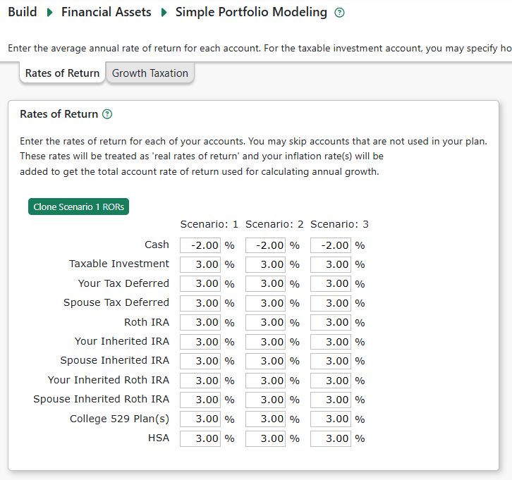
NOTE: Pralana rebalances your portfolio every year in seeking to maintain the asset locations specified in this table.
When using Mode 1, you should be aware that your overall asset allocation can change as your account balances change, but it can be viewed on the Review > Tabular Projections > Portfolio > Allocations tab. To maintain a consistent overall allocation, you would need to use the same asset location settings on all accounts. If you want to vary your overall asset allocation over time, you can simply specify different asset locations in multiple periods.
Mode 2: Portfolio Allocation
This tab appears only when that Mode 2 is selected. On this page, Pralana shows columns for:
the overall portfolio allocation for each asset class
column for the target asset location for each account, except the Cash account which is always 100% allocated to the Cash asset class.
There will be rows for each of your asset classes in each portfolio time period. Enter the overall portfolio asset allocation you wish to achieve as well as the target asset locations for each of your accounts, ensuring that all the column totals are 100%.
Pralana can model variations in your global asset allocations and asset locations over time. To enable this, for each time period identified on the Portfolio Time Periods subpage of the Build > Financial Assets > Advanced Portfolio Modeling page, Pralana replicates the table containing a row for each asset class and a column for each account, along with an indication of the related start year. To model different allocations over time, just modify the values in the allocation and location columns as desired.
Here is an example of the set-up of this tab:
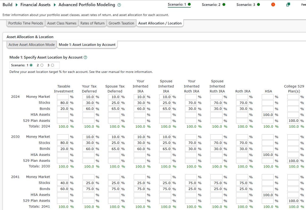
Important: The Mode 2 actual account asset locations will likely vary every year, and be different from your account target asset locations. Consider Mode 2 like a school cafeteria lunch operating first-come, first-served:
Say there are two menu selections (aka asset classes): Hot Dogs and Hamburgers and each of the 100 kids (accounts) gets one.
Suppose the ‘overall allocation’ is 50% hot dogs 50% hamburgers, so the staff prepares 50 hot dogs and 50 hamburgers.
But, suppose 60% of the kids want a hot dog (their target allocation is 100% hot dogs).
Well, the first 50 kids in line (by ‘kid prioritization’) will get what they want…either a hot dog or hamburger.
At some point the remaining 10 kids that want hot dogs get served and find there are no hot dogs left. They get a hamburger.
Similarly, in Mode 2, your total portfolio’s starting balance and overall target asset allocation determine how much of each asset class is available to distribute among your accounts for the year. Assets are then assigned to accounts in the order of your Mode 2 Account Prioritization. The highest-priority account is processed first and receives its target allocation based on its starting-year balance. Then, the next account in the priority list is processed, and so on. As each asset class’s available “pool” is used up, that class becomes unavailable for subsequent accounts. Lower-priority accounts therefore receive allocations only from whatever assets remain.
You can view the actual allocations on the Review > Tabular Projections > Portfolio> Allocations tab.
Mode 2: Account Prioritization
This tab enables the prioritization of your accounts for the Mode 2 asset allocation process. The table on this tab shows all your accounts arranged from top to bottom in priority order. To change the priority, simply left click (i.e., click and hold) on an account, drag it to the desired position and then unclick. Repeat this process with other accounts until the table is in the desired order. Be aware that this order applies to all time periods.
Here is an example of the set-up of this tab:
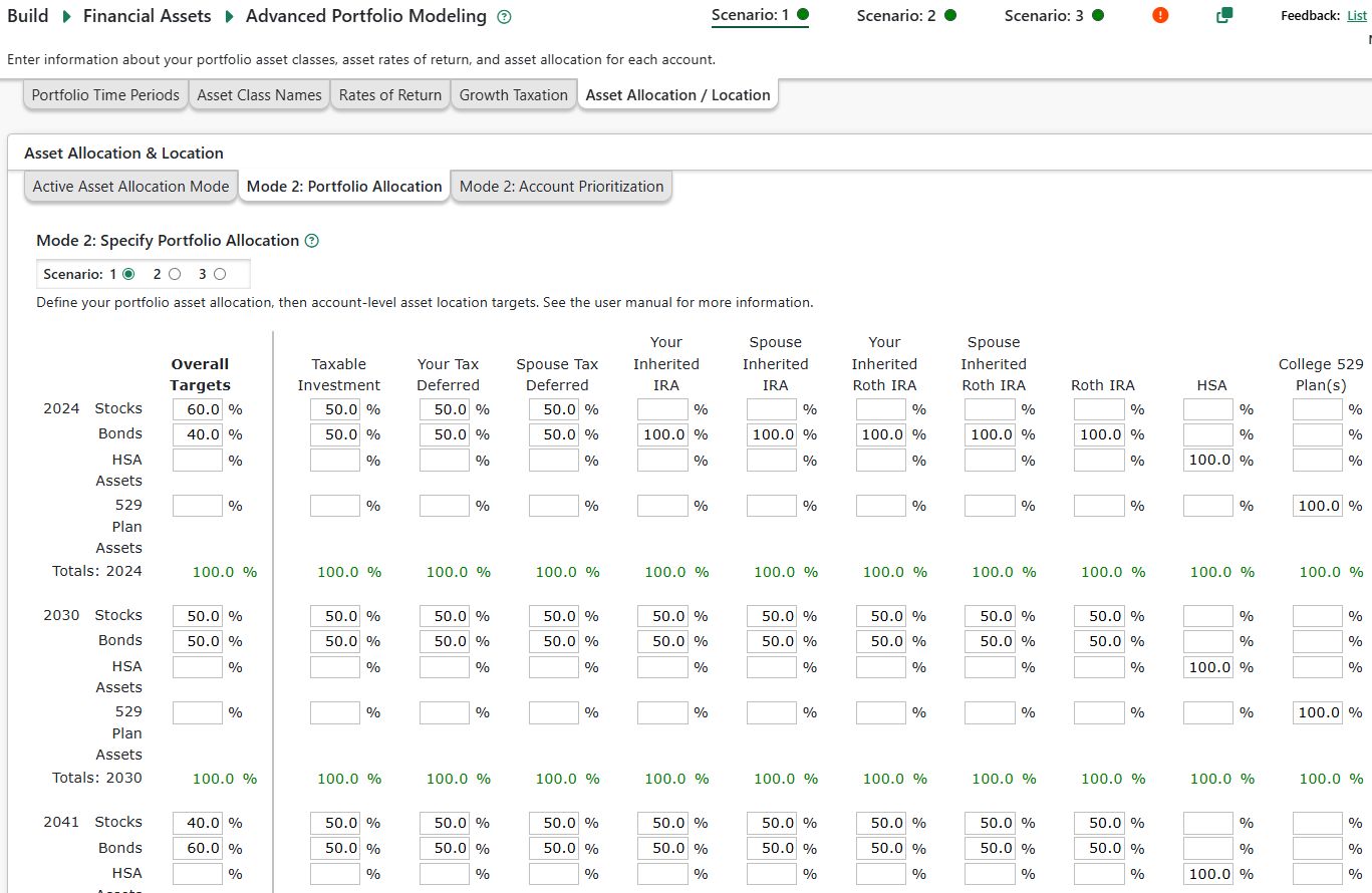
Overall allocation vs. What-If Savings Projection Graph
On the Review > Graphical Projections > Asset Allocation page, Pralana presents a graph that enables you to see the calculated overall allocations immediately (based on a deterministic projection), juxtaposed with the corresponding savings projection for the selected scenario.
Taxable Investment Account: Allocate Initial Unrealized Long Term Capital Gains
On the Initial Balances Page, you may specify the amount of unrealized long-term capital gains (LTCG) held in your taxable investment accounts. For the Taxable Account, Pralana tracks the amount of unrealized by asset class. Thus, it is necessary to know how your total initial unrealized LTCG is allocated between your asset classes at the start of your plan.
The input table lists the asset classes allocated to your Taxable Investment account in the first plan year and, for each, the allocation percentage and amount. By default, the unrealized LTCG allocation matches your asset allocation. However, you should review and update the allocations as cash equivalent and fixed income asset classes are likely to have a little unrealized LTCG while stocks and other equity assets are likely to hold most of the unrealized LTCG.
As you edit the LTCG allocation percentages, Pralana will update the dollar amount of unrealized LTCG by asset class in the right-most column.
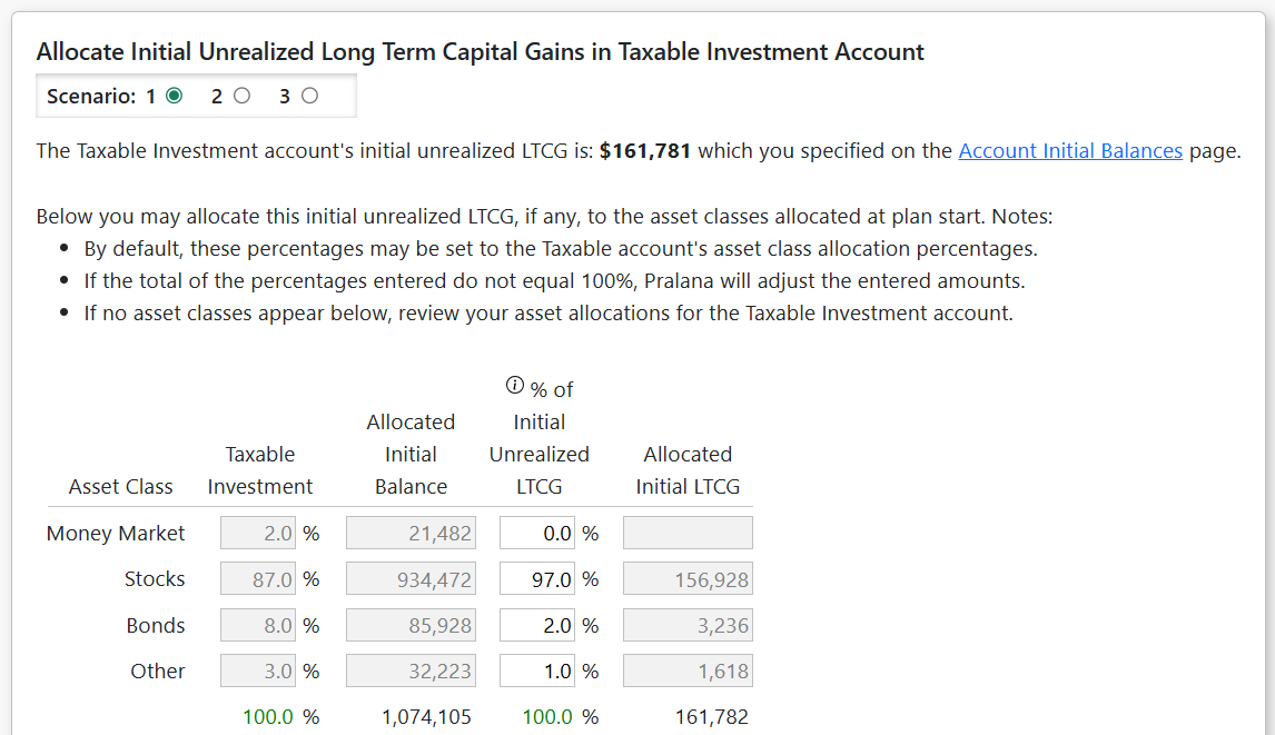
Asset Allocation Tabular Projection
You can view the actual allocations on the Review > Tabular Projections > Portfolio> Allocations tab.
When using Advanced Portfolio Modeling, Mode 2: Specify Overall Allocation, you may want to exclude the Cash, HSA and 529 Plan accounts from the Overall totals. These are excluded from the Mode 2 allocation process but will be included in the Overall totals unless you choose to exclude them. The Cash account is always 100% allocated to cash and the HSA and 529 plans always get the asset allocation you specify. Some accounts may not receive their target allocations. For an explanation, see section ‘Mode 2: Portfolio Allocation’ above.
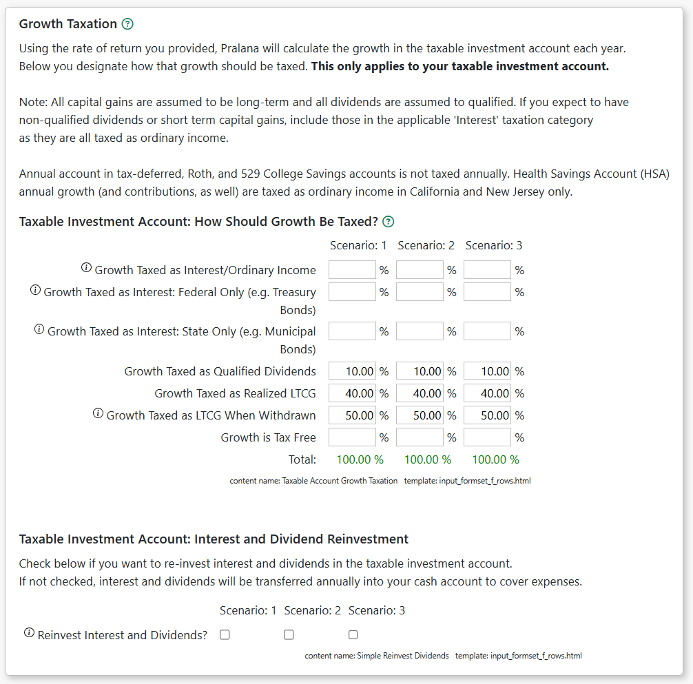
The Effective Buying Power of Your Portfolio
You should be cautious when comparing the value of a portfolio where investments are held mostly in taxable or tax-free accounts with one where investments are held mostly in tax-deferred accounts because the funds in tax-deferred accounts are not all yours. Some of that money belongs to Uncle Sam; he just has not collected it from you, yet. To help you with this, Pralana calculates the effective buying power of your portfolio as a function of its distribution across accounts with differing taxation properties. Money held in Cash, Taxable and Roth accounts is counted at full value; money held in the Tax-Deferred accounts is derated based on the Effective Tax Rate you expect to apply to those funds when withdrawn. If you plan to leave some or all your tax-deferred accounts to your heirs, the withdrawals are likely to be different than your own tax rates. Therefore, Pralana asks you to specify the effective tax rate to be used when determining the effective buying power of those accounts. To do this, go to the Build > Financial Assets > Management > Effective Tax Rate page and enter the desired rate to be used for this conversion process.
The Roth conversion optimization algorithm uses your effective total savings in the determination of the optimum Roth conversion parameters and the graphical display on the Analyze > Roth Conversions page presents a comparison of your baseline plan and your “what-if” plan in terms of either effective dollars or absolute dollars. Just click the button beneath the graph to switch between these options.
Modeling Scheduled Withdrawals
The Build > Financial Assets > Scheduled Withdrawals page allows you to define withdrawals/transfers from any account to any other account (except inherited IRAs) or to an external (out of plan) destination. Transfers from an IRA to the Roth account should be done on the Roth Conversions page and not as a Scheduled Withdrawal.
Scheduled withdrawals provide a mechanism for:
funding certain expenses out of specific accounts,
modeling HSA reimbursements
closing out or transferring excess 529 college savings plan funds
gifting appreciated assets without triggering an asset sale and capital gains taxes
Notes:
Withdrawals will be reduced or eliminated if the source account has insufficient funds in the withdrawal year. If this occurs, an alert will be created.
Transfers into HSAs and pre-tax transfers into IRA’s are Federal and state tax-deductible (except NJ and CA). These transfers are shown on Form 1040 Schedule 1 Part II ‘Adjustments to Income’: line 13 ‘Health savings account deduction’ and line 20 ‘IRA deduction’.
Inputs
Source Account: Select the source account. For some accounts you will have the option to indicate whether the withdrawal is subject to penalty and for IRA’s whether the withdrawal is tax-exempt. It is your responsibility to determine whether you are eligible to make the withdrawal/transfer in the specified year and amount.
Destination Account: Select the destination account. For IRA’s you may specify whether the amount transferred is pre-tax or after-tax dollars. If you need to transfer both, set up two transfers. If the destination is “External (out of plan)” Pralana will transfer the amount without triggering an asset sale. If the source is the Taxable Investment account, unrealized long-term capital gains will be reduced by a pro-rated amount of the withdrawal amount and the account’s % unrealized LTCG in that year.
Amount: Enter the withdrawal amount in today’s dollars. Pralana will inflate the amount from the plan start year to the withdrawal year using your inflation rate.
Start Year: Enter the year the withdrawal(s) are to begin.
End Year: This is the last year of the withdrawals. For one-time withdrawals, set this equal to the Start Year. For indefinite withdrawals, leave this field blank.
Description: a brief description of the planned withdrawal for your use only.
Using Scheduled Withdrawals for LTCG Harvesting (Taxable → Taxable)
You may specify a Scheduled Withdrawal from the Taxable Investment account back into the Taxable Investment account. This will force a sale of assets to cover the withdrawal. For simplicity, Pralana assumes that asset classes are sold in proportion to their allocation. Within each asset class, LTCG is realized per your LTCG Withdrawal Strategy.
Note: realized LTCG is taxable, though often at lower rates than ordinary income. In years of low ordinary income, the realized LTCG may be taxed at the 0% or 15% rate. This is an advanced topic requiring close attention.
Using Scheduled Withdrawals to Minimize the Effects of Unscheduled Withdrawals
As discussed in the section of Unscheduled Withdrawals and Iterative Tax Calculations, any negative cash flows that result in unscheduled withdrawals from tax-deferred accounts are included in the AGI for the subsequent tax year. The same is true for LTCG on unscheduled withdrawals from the taxable account. If this situation occurs in your scenarios for relatively few years, you may consider setting up scheduled withdrawals to offset and eliminate those negative cash flows. That will eliminate the unscheduled withdrawal and the deferral of the associated taxes to the next year, thereby improving the accuracy of the model in the near term. Please note: when same-year taxation of unscheduled withdrawals is implemented this issue will cease to exist.
Modeling Substantially Equal Periodic Payments (SEPPs)
The Build > Financial Assets > SEPPs page implements Internal Revenue Code (IRC) section 72t, which allows early withdrawals from tax-deferred (TD) accounts without the normal 10% penalty. SEPP payments are computed by one of three methods (amortization, annuity or minimum distribution) and run for five years or until the owner reaches age 59, whichever occurs latest. The IRS does not allow SEPP payments from qualified retirement plans while you are still employed by the associated plan sponsor, but Pralana does not enforce any such rules. You should research IRC section 72t yourself to ensure your understanding of all the rules. Pralana allows you to specify one SEPP period for your TD account and another for your spouse’s. It also allows you to specify one of two payment calculation methods: fixed or RMD. The amortization and annuity methods both result in fixed payments, so Pralana simplifies the process by just asking you to specify the amount in terms of today’s dollars. The minimum distribution method calculates the amount based on account balance and the owner’s life expectancy according to IRS mortality tables. Withdrawal amounts are treated like RMDs: they are taxed as ordinary income and deposited in your cash account and if this causes that account to exceed its ceiling level the balance will be deposited in the regular investment account.
Modeling Charitable Trusts
NOTE: As of Dec 2025, the Charitable Trusts feature has not yet been implemented.
The Build > Financial Assets > Charitable Trusts page allows you to set up the modeling of the funding and payouts from a charitable trust. Pralana does not attempt to model the details of specific types of trusts but, rather, provides the basic controls through which you can tailor its capabilities to a variety of trust types and details. Pralana does not maintain the balance of the trust but it does model the establishment of a trust in the past or future, along with subsequent tax deductions and annuities (i.e., payouts). The contribution amount will always be withdrawn from the regular investment account. The deductions and payouts can vary every year, so Pralana simply provides you with a table through which you can manually specify the annual amounts. The deductions will be included in your itemized deduction calculations, and the payouts will be taxed as ordinary income.
Modeling Your Personal and Investment Loans
Personal Loans
On this page, you can define personal loans you have made in the past or will make in the future. The outstanding loan balance of personal loans is included in your Net Worth.
Loan input fields vary depending on whether the loan was originated prior to the plan start year (existing loans) or in/after the plan start year (future loans). Fields with a blue background are required. Fields that are informational or not applicable will be greyed out and not editable.
Inputs
Description: Enter a description or other notes about the loan (up to 255 characters).
Origination Year: Enter the loan’s origination year. This year, along with your plan start year, determines whether the loan is a past or future loan.
Interest Rate: Enter the annual interest rate.
Term: Enter the loan’s term in years. This is optional for loans originated in the past (unless the loan has an interest only period) because Pralana will calculate the amortization using the Interest Rate, Balance at Plan Start, and Monthly Payment.
Balance at Plan Start: For existing loans enter the outstanding loan balance as of the plan start date. This field is disabled for future loans.
Monthly Payment: For existing loans, enter the loan’s monthly principal and interest payment.
Loan Amount: For future loans, enter the anticipated loan amount in today’s dollars.
% of Interest Received Taxable: Enter the percentage of the loan interest received that is taxable. The default is 100%.
% of Principal Received Taxed as LTCG: Enter the percentage of the loan principal received that is taxable as a long-term capital gain. The default is 0%. This field may be applicable if, for example, you sold a business and provided financing to the buyer.
Optional Loan Fields
All loans have these optional fields which are less commonly used. Click the Show Optional Fields checkbox to reveal these fields.
Interest-Only Period: You may specify an interest-only period, in years. The interest only period starts in the origination year. During the interest-only period, Pralana will calculate and apply the interest-only payment and the loan’s principal balance will remain unchanged (unless you also specify an additional principal payment). After the interest only period:
For existing loans, Pralana will use your entered monthly payment to amortize the loan until it is paid off.
For new loans, Pralana will calculate the monthly payment required to amortize the loan balance from the start of the repayment period until the end of the remaining loan term.
Early Pay-Off Year: If you specify an early pay-off, the loan balance (at the end of the prior year) will be paid-in-full at the start of this year. The lump-sum payoff amount will be shown on the amortization schedule and treated as income in the pay-off year.
Extra Principal Payments (Annual $): You may specify additional principal payments by entering an annual amount. Pralana will apply these additional principal payments in the years specified (but not prior to plan start).
Extra Principal Payments Start: Enter the year you plan to start making the excess payments. For existing loans, Pralana assumes that any additional principal payments may in the past are reflected in the Balance at Plan Start field.
Extra Principal Payments Stop: Enter the year you plan to stop making excess payments (i.e., the last year of those payments). Leave this field blank if you intend to make the extra payments until the loan is paid-in-full.
Amortization
This tab shows the amortization of your personal loans. The total balance of the loans modeled on this page will included as “Balance on Personal Loans Made By You” in the Other Assets section of the Balance Sheet and add to your net worth.
Investment Loans
On this page you can model loans that are not specifically associated with the purchase of physical property, such as investment or margin loans.
Loan input fields vary depending on whether the loan was originated prior to the plan start year (existing loans) or in/after the plan start year (future loans). Fields with a blue background are required. Fields that are informational or not applicable will be greyed out and not editable.
Inputs
Description: Enter a description or other notes about the loan (up to 255 characters).
Origination Year: Enter the loan’s origination year. This year, along with your plan start year, determines whether the loan is a past or future loan.
Interest Rate: Enter the annual interest rate.
Term: Enter the loan’s term in years. This is optional for loans originated in the past (unless the loan has an interest only period) because Pralana will calculate the amortization using the Interest Rate, Balance at Plan Start, and Monthly Payment.
Balance at Plan Start: For existing loans enter the outstanding loan balance as of the plan start date. This field is disabled for future loans.
Monthly Payment: For existing loans, enter the loan’s monthly principal and interest payment.
Loan Amount: For future loans, enter the anticipated loan amount in today’s dollars.
% of Tax Deductible: Enter the percentage of the loan interest received that is tax-deductible. The default is 100%.
Optional Loan Fields
All loans have these optional fields which are less commonly used. Click the Show Optional Fields checkbox to reveal these fields.
Interest-Only Period: You may specify an interest-only period, in years. The interest only period starts in the origination year. During the interest-only period, Pralana will calculate and apply the interest-only payment and the loan’s principal balance will remain unchanged (unless you also specify an additional principal payment). After the interest only period:
For existing loans, Pralana will use your entered monthly payment to amortize the loan until it is paid off.
For new loans, Pralana will calculate the monthly payment required to amortize the loan balance from the start of the repayment period until the end of the remaining loan term.
Early Pay-Off Year: If you specify an early pay-off, the loan balance (at the end of the prior year) will be paid-in-full at the start of this year. The lump-sum payoff amount will be shown on the amortization schedule and treated as an expense in the pay-off year.
Extra Principal Payments (Annual $): You may specify additional principal payments by entering an annual amount. Pralana will apply these additional principal payments in the years specified (but not prior to plan start).
Extra Principal Payments Start: Enter the year you plan to start making the excess payments. For existing loans, Pralana assumes that any additional principal payments may in the past are reflected in the Balance at Plan Start field.
Extra Principal Payments Stop: Enter the year you plan to stop making excess payments (i.e., the last year of those payments). Leave this field blank if you intend to make the extra payments until the loan is paid-in-full.
In the year the loan is originated, the loan amount will be added to your Taxable Investment Account and all loan expenses will be shown in the corresponding column on the Review > Tabular Projections > Expenses page. If the term of the loan is the same as the interest-only period, a balloon payment will be generated in the last year of the loan. If the Tax Deduction box is checked, the interest on the associated loan will be included in the Deductions and Exemptions column on the Review > Tabular Projections > Expenses > Taxes > Itemized Deductions page.
Amortization
This tab shows the amortization of your investment loans. The total balance of the loans modeled on this page will be included as “Investment Loan Balance” in the Liabilities section of the Balance Sheet and reduce your net worth.
Modeling Your Taxes
Pralana performs detailed tax calculations, though it does not implement the entire Federal tax code nor the entire tax codes of any State. These are detailed approximations only, but the tool does give you the ability to view some of the key tax forms to help you understand how its numbers are derived. Please visit the Review > Reports > Tax Forms page and you can then scroll through the forms for any selected year.
Federal Income Tax and Alternative Minimum Tax
Federal income taxes, including the Alternative Minimum Tax (AMT), are calculated automatically by Pralana and are based on the following:
Adjusted Gross Income (AGI), the details of which are shown on the AGI Details tab of the Review > Tabular Projections > Taxes page
Long term capital gains or losses
Capital loss carryover
Marital status and number of dependents
Tax law in effect (either TCJA of 2017 or pre-TCJA of 2017)
Standard deduction or itemized deduction, whichever is larger (itemized deduction details are shown on the Itemized Deductions tab of the Review > Tabular Projections > Expenses > Taxes page
Exemptions
Current federal tax tables (indexed for inflation in future years)
Child tax credits
You can see the details on the Taxes tabs of the Review > Tabular Projections > Expenses page and the Review > Reports > Tax Forms & Brackets page.
State Income Tax
State income tax is calculated automatically by Pralana and is based on the following:
Marital status and number of dependents
State of residence
Federal AGI
Standard deductions
Whether or not the following items are deductible in your state of residence and any individual or family limits on these:
Social Security income
Distributions from retirement accounts
Pensions, with differentiation between private, military and government pensions
Interest and dividends
Earned income
Federal income taxes
2023 tax tables (indexed for inflation in future years)
You can see the details on the Taxes tabs of the Review > Tabular Projections > Expenses page and the Review > Reports > Tax Forms page.
State income taxes are particularly difficult to model, with 51 sets of rules (50 states plus the District of Columbia), so it is possible that the model is not always accurate for your case. If this algorithm does not seem to be calculating state taxes correctly for your case, you can use the alternative method provided here: On the Residence/Relocation tab of the Build > Get Started > Scenario Assumptions page, simply specify a rate that Pralana will multiply by the federal AGI to arrive at an estimate of your state income taxes. This alternative method will replace the detailed calculations if this field contains any data.
Please note: If you do discover that Pralana is producing inaccurate values for the taxes in your state we will always welcome an email to provide us with the details so that we can continue to improve the model.
Local Income Tax
Pralana can estimate local income tax each year based on inputs provided by you on the Scenario Assumptions > Residence/Relocation page:
Local Tax Rate: Enter a percentage representing the locality’s tax rate to be applied to the Local Taxable Income choice you make.
Local Taxable Income: Select from these 3 choices. For each state, Pralana will indicate which taxable income is the default (most commonly used).
Federal Taxable Wages (for localities that tax only earned income)
Federal Adjusted Gross Income
State Taxable Income
Payroll Taxes
Pralana calculates FICA taxes separately for both marital partners based on their respective income streams. Self-employment income is treated appropriately and applicable annual maximums are used in these calculations. In Pralana, payroll taxes are considered adjustment to spendable income. See “Payroll Taxes” column at Review > Tabular Projections > Income > Income Statement (click for Metric MRI) as well as Review > Tabular Projections > Taxes > Summary (Payroll Taxes section).
Net Investment Income Taxes
Pralana calculates Net Investment Income Taxes (NIIT) automatically based on your AGI and investment income. See how NIIT is calculated on Form 8960 in the Tax Forms.
Performing Deterministic, Monte Carlo and Historical Analysis on Your Plan
In this section, we will discuss the Basic Analysis of your plan. Your basic assumptions, income, expenses and financial assets have already been entered to establish a Base Plan and now it is time to take a look at the prognosis. Based on the results of those analyses, you can go back and adjust your initial inputs or proceed on to more detailed analyses.
Since some variables are unknowable (most notably: life expectancy, inflation, and rates of return (ROR) on investments), no calculator can produce a single “right answer” regardless of the amount of detail you put into it. Further, the long-term growth of investments is a function of market volatility and the sequence of returns. In other words, year to year variations in ROR can make a big difference in the size of your savings accounts over time. Here is one simple example to illustrate the point: A 10% loss one year followed by a 10% gain the following year is really a 1% loss over that two-year period. A $100,000 portfolio would be reduced to $90,000 after the first year and would rise to $99,000 after the second year for a loss of $1000, or 1%. Even though the average return in this example is 0%, if this portfolio experienced a constant 0% return over that same period, it would still be worth $100,000 and, thus, ahead of the same portfolio that experienced the volatility.
To address these uncertainties, Pralana analyzes your data using three different analysis methods (deterministic, Monte Carlo and historical) to provide you with a range of likely outcomes.
Deterministic Analysis
Pralana’s deterministic analysis generates a single projection using an average inflation rate and average rates of return each year, as specified on the Build pages. This is the most basic form of financial analysis and is particularly useful for getting a general understanding of where you stand relative to long term objectives, for making trade-offs between major choices and for exploring the sensitivity of your plan to certain parameters, such as inflation, rates of return, life expectancy, and so on. Its primary weakness is that it does not model year-to-year fluctuations in rates of return and inflation, which are facts of life in the real world. Consequently, the probability that your actual long-term results will be better than those predicted by fixed rate projections are (very roughly) 50%, but the probability that you will do worse are also (very roughly) 50%. The screenshot below was taken from the Analyze > Historical Analysis page; the red line shows the deterministic projection juxtaposed with historical analysis results, and you can see the same red line juxtaposed with Monte Carlo analysis results on the Analyze > Monte Carlo Analysis page.
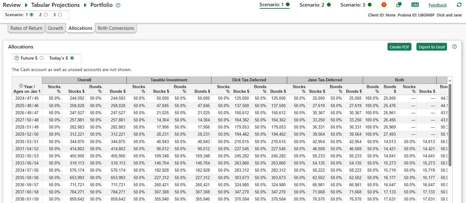
To view the results of Pralana’s deterministic analysis results in tabular form, go to the Review > Tabular Projections pages. To see a detailed graphical breakdown, go to the Review > Graphical Projections pages. All the data presented on those pages is based on a deterministic analysis UNLESS the Historical Sequence Analysis has been activated on the Analyze > Historical Analysis page. There are a variety of pages available designed to give you functionally coherent insights into Pralana’s deterministic projections.
Tabular Projections
Pralana presents a robust set of tabular deterministic analysis outputs accessible via the Review > Tabular Projections pages. These pages show year-by-year deterministic projections for the scenario selected via the radio buttons at the top of the page. All data can be viewed in either future dollars or today’s dollars based on radio buttons located directly above the tabular data, and data columns containing only zeroes can be hidden as a function of the setting of a check box just above the tabular data.
If the Historical Sequence Analysis is active (which is controlled via a checkbox on the Analyze > Historical Analysis page), you can examine the year-by-year projection details via the Tabular Projections pages, and a banner will be displayed in the upper right corner of each page as shown in the screenshot below:
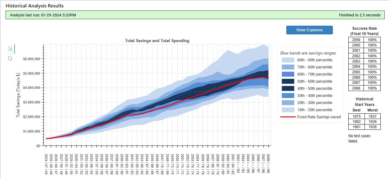
Tabular projections are presented by topic, as follows:
Income, with different tabs for Income Statement, Income Details, and Payroll Contributions
Expenses, with different tabs for Expense statement, Expense details, and Taxes
Cash Flow, with different tabs for Cash Flow Statement, Withdrawals, and Annuity Purchases
Balance Sheet
Portfolio, with different tabs for Rates of Return, Growth, Allocations, and Roth Conversions
Account Statements
Scenario Assumptions
On all these pages, the first column contains three numbers separated by a “/”. The 4-digit value is the year, the first 2-digit value is your age as of January 1 in that year and the second 2-digit value is your spouse’s age as of January 1 in that year. That column will remain fixed as you scroll left and right.
The data presented on the tabular projection pages will be updated anytime you make a change to your plan via one of the Build pages.
Today’s Dollars vs. Future Dollars
Tabular projections can be calibrated in terms of future dollars or today’s dollars. When the projections are presented in terms of today’s dollars, the data will be adjusted for inflation. Consequently, outputs that increase at the rate of inflation will appear as constant values. For example, if you have an income of $100,000 per year that increases at the same rate as inflation, it will appear as $100,000 every year. Conversely, if inflation is 3%, that same income stream presented in terms of future dollars will begin at $100,000, and then increase to $103,000 in the second year, to $106,090 in the third year, and so on.
Metric MRI
For some complex metrics, Pralana includes a feature called Metric MRI which, like medical magnetic resonance imaging, provides a look ‘inside’ the metric to see how it was calculated.
Click underlined metrics in some tabular projections to open the Metric MRI, a pop-up audit of the metric. Metric MRI is currently available for Social Security income, account growth and balances, Healthcare and Medicare costs, Roth conversion amounts, etc. Additional metrics will be supported in the future based, in part, on user interest.
The pop-up Metric MRI box may be moved and resized with your mouse or touchpad. Close it by clicking the X at the top right.
Income
This page includes three tabs: Income Statement, Income Details, and Payroll Contributions. The income statement shows a summary of all your income sources and any adjustments to your income (such as payroll taxes and contributions) in one view, and ultimately getting to your spendable income each year. The income details tab shows an elaboration of the income sources shown on the income statement tab, and the payroll contributions tab shows an elaboration of the payroll contributions shown on the income statement tab. Please note that this does NOT include everything the IRS taxes as income: RMDs, for example, are taxed as ordinary income but they are not true income and are shown as a “cash inflow” in the Cash Flow statement.
Expense
This page includes three tabs: Expense Statement, Expense Details, and Taxes. The Expense Statement tab includes a column for each type of expense as specified on the Build > Expenses pages as well as columns for taxes, and ultimately getting to your total expenses. When you select the Expense Details tab, you will then see separate tabs for each type of expense that you can specify on one of the Build > Expenses pages, and these tabs will present your expenses in detail. When you select the Taxes tab, you will then see separate tabs for your taxes, a detailed breakdown of your Adjusted Gross Income (AGI), and a detailed breakdown of your itemized deductions.
Cash Flow
The Cash Flow page includes three tabs to show you the movement of money within your portfolio: Cash Flow Statement, Withdrawals and Annuity Purchases. The cash flow statement shows all the cash flowing into the cash account (referred to as Cash Inflows), your Total Expenses as elaborated on the Expense Statement, your net cash flow, the starting and ending cash account balance, and the money transferred out of the cash account to your taxable investment account and the money transferred into the cash account from your other accounts to cover periods of deficit spending.
All positive and negative cash flows will be applied to your cash account, in turn driving that account’s balance up or down; however, as explained in the Financial Assets > Management section above, you can specify floor and ceiling amounts for your cash account, and these levels are adjusted annually for inflation. All negative cash flows are taken from the cash account until the floor is reached, and thereafter the withdrawal priority order is used to determine the account to be used to cover the remaining portion of the negative cash flow; all positive cash flows as well as withdrawals and distributions from tax-favored accounts are deposited in the cash account until the ceiling is exceeded, after which the excess is transferred to the taxable investment account.
The Withdrawals tab shows the details of all scheduled and unscheduled withdrawals from each of your accounts. The Annuity Purchases tab shows the purchase of annuities and the account from which the purchase was made.
Balance Sheet
This page presents a year-by-year summary of all your account balances, your other assets, your liabilities and your net worth. All account balances can be clicked to bring up the Metric MRI window to show you how the balance in any year has been computed. Here is an example:
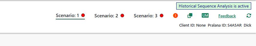
Portfolio
This page includes four tabs: Rates of Return, Growth, Allocations, and Roth Conversions. The Rates of Return tab shows the ROR for each of your accounts and the Growth tab shows the corresponding annual growth of each account as the result of applying the ROR. The Allocations tab shows your overall asset allocation and the allocation of each asset class to each of your accounts. If you are using the Simply Portfolio Modeling option and are specifying account RORs directly, then the Allocations tab will simply show what portion of your portfolio is associated with each account, along with each of your account balances. If you are using the Advanced Portfolio Modeling option, the Allocations tab will show the annual allocation to each of your asset classes as well as the portion of each account assigned to each asset class and the corresponding dollar amounts.
Account Statements
For each of your accounts, this page shows the year-starting balance, all the deposits and withdrawals, and the year-ending balance. This should make clear what is driving the account balances from year to year. When viewing the data in terms of today’s dollars, inflation adjustments are applied on the first tick of the clock in the year. Consequently, the Ending Balances are not discounted for the duration of the year and will not match the Starting Balance shown for the next year or the corresponding ending balance on the Balance Sheet.
Unused accounts are not shown. The Starting Balance and Ending Balance rows cannot be hidden.
Scenario Assumptions
This page shows you the general inflation rate, the cumulative inflation, your tax filing status and your state of residence for each year in the modeling period.
Graphical Projections
Pralana generates two different forms of detailed graphical projections of deterministic analysis results which are naturally consistent with the data in the tabular projections described in the previous section:
Savings and Net Worth
Cash Inflows
Taxes
Asset Allocation
Key Metrics by Scenario
Savings & Net Worth
This page presents a graph of your savings and net worth juxtaposed to your income and expenses for the active scenario. The bar graphs show the distribution of your savings and net worth across your various accounts and properties, while your income and expenses are shown via line graphs. The bar graphs are calibrated against the vertical axis on the left and the line graphs are calibrated against the vertical axis on the right.
Cash Inflows
This chart illustrates the Cash Inflows section of the Cash Flow Statement. It shows the components of Spendable Income plus other sources of cash. The total of these metrics is Total Cash Inflows which, along with Total Cash Outflows, is used to determine Net Cash Flow each year.
Tax Projections
This page contains several tax-related graphs for the active scenario.
Tax Brackets:
Ordinary Income: Shows your taxable ordinary income vs the Federal ordinary income brackets.
Long Term Capital Gains: Shows your taxable income (upper line) and ordinary income (lower line) vs the Federal LTCG brackets. The blue-shaded area is taxable LTCG and qualified dividends.
Medicare IRMAA: Shows your Medicare Modified Adjusted Gross Income (MAGI) vs the Medicare IRMAA brackets. The MAGI amount shown for each year is based on Federal AGI
from the 2nd prior year due to the 2-year lookback.
Taxes by Type: A bar chart showing taxes by year, split between Federal income tax, state and local income tax and Social Security / Medicate wage taxes.
Key Inputs to Tax Calculations: A line chart showing the key metrics used in calculating federal income tax.
Portfolio Asset Allocation
This page shows a graphical projection of the allocation of your portfolio to your asset classes over the modeling period. If you are using Simple Portfolio Modeling, this graph will show the percentage of your portfolio associated with each of your accounts. If you are using Advanced Portfolio Modeling, this graph will show the percentage of your portfolio associated with each of your asset classes.
Compare Key Plan Metrics by Scenario
This page shows a line graph with your savings balances and expenses from all three scenarios overlaid for easy comparison. You can hide or show any of the lines to focus on any specific comparison of your choice. Here is an example:
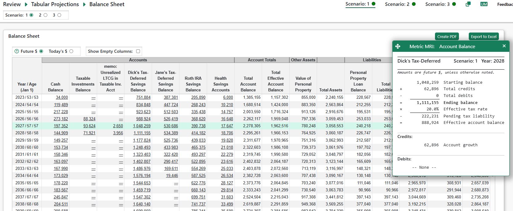
Monte Carlo Analysis
Pralana’s Monte Carlo analysis generates 1,000 long-term projections to model the impact of market volatility on your financial plan. Each projection represents a plausible future path for investment returns, allowing you to assess the range of possible outcomes rather than relying on a single deterministic forecast.
All projections use the same inflation assumptions, income profile, and non-tax expenses as the deterministic analysis. Investment returns vary across projections, and as a result, taxes may also vary because they depend on realized returns.
In Monte Carlo analysis, Pralana applies randomly varying rates of return (RORs) to your financial assets. The random returns are based on your specified account-level or asset-class rates of return, converted to nominal rates if needed, and then randomized using either:
Pralana’s default standard deviation, or
Custom standard deviations that you define on the Monte Carlo Analysis page.
Pralana uses arithmetic returns for Monte Carlo modeling and supports either correlated or uncorrelated asset classes, based on your selections.
Monte Carlo Results
The Monte Carlo chart shows both the results of the Monte Carlo analysis
and (optionally) how the scenario has changed since the analysis was
last run. 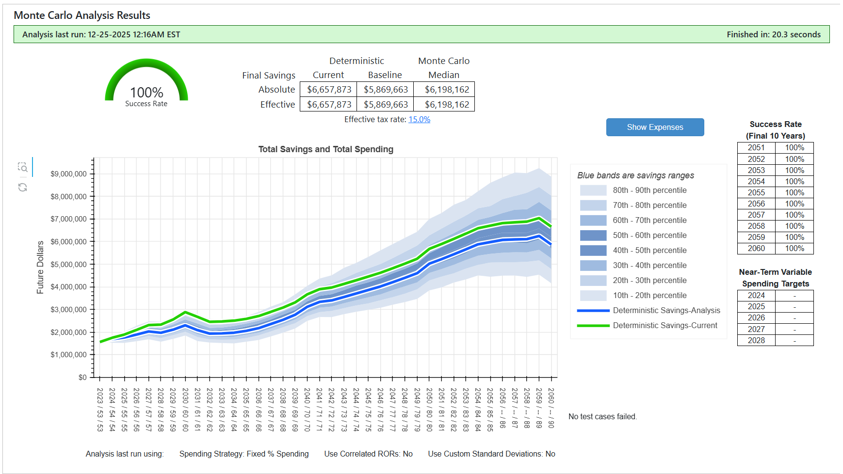
Blue shaded bands: Monte Carlo savings distribution
The blue shaded bands represent the distribution of projected total savings produced by the 1,000 Monte Carlo runs:
The bands show the range of outcomes for the 2nd through 9th deciles (i.e., the middle 80% of results).
Wider bands indicate more dispersion (uncertainty) in outcomes.
Blue lines: scenario values at analysis time
When you run Monte Carlo, Pralana captures the scenario’s deterministic projections at that moment and plots them in blue:
Blue solid line: deterministic total savings at the time the analysis was run
Blue dashed line (when shown): deterministic total expenses at the time the analysis was run
These blue lines provide a baseline reference so you can compare the Monte Carlo outcome distribution to the deterministic projection at the time (shown in the status bar) the analysis was executed.
Green lines: current scenario values (after changes)
After running Monte Carlo, if you change inputs that affect the scenario projection, Pralana will display green lines to show the current deterministic projection:
Green solid line: current deterministic total savings (based on the updated inputs)
Green dashed line: current deterministic total spending/expenses (based on the updated inputs)
These green lines make it easy to see how your changes would affect the deterministic projection relative to the Monte Carlo results and the deterministic baseline that existed when the analysis was run.
Tip: If you have changed inputs since the last Monte Carlo run, the green lines reflect your current scenario, but the shaded Monte Carlo bands still reflect the analysis results from the last run. Re-run Monte Carlo to update the bands to match your latest inputs.
User Controls
Pralana gives you control over two important aspects of the Monte Carlo analysis:
Whether the randomized asset class rates of return are assumed to be correlated or uncorrelated.
The standard deviation associated with the rates of return specified on the Build > Financial Assets > Asset Classes page.
These settings influence the amount of variability and diversification reflected in the Monte Carlo results.
Standard Deviation
Standard deviation measures how much investment returns are expected to vary around their average value. Higher standard deviation implies greater volatility and a wider range of possible outcomes.
In the Monte Carlo analysis, Pralana generates random rates of return for each asset class using a normal distribution defined by:
The average rate of return you specify, and
An associated standard deviation.
If you are using Advanced Portfolio Modeling, Pralana provides two ways to specify standard deviation values, selected using the checkbox on the Analyze > Monte Carlo Analysis page.
1. Calculated default standard deviation (Checkbox unchecked)
Pralana automatically assigns a standard deviation to each asset class using a simple rule:
Standard deviation = geometric nominal rate of return × 1.5
This approach avoids the need to research and select volatility assumptions while producing reasonable, historically grounded values. For example:
U.S. stocks:
Long-term average return ≈ 11%,
historical standard deviation ≈ 19%
Pralana default standard deviation ≈ 16.5%
10-year Treasury bonds:
Long-term average return ≈ 4.8%,
historical standard deviation ≈ 7.5%
Pralana default standard deviation ≈ 7.2%
These values are intended as practical approximations rather than precise historical matches.
2. Custom standard deviation by asset class (Checkbox checked)
You may instead specify standard deviation values directly. For each time period defined on the Advanced Portfolio Modeling page, the Rate of Returns Std Deviations tab displays a row for each asset class, allowing you to enter a custom standard deviation for that period.
This option is intended for advanced users who want direct control over volatility assumptions.
Interpreting Volatility Assumptions
Assets with higher expected returns generally exhibit higher volatility. Conservative return and volatility assumptions will result in a narrower range of Monte Carlo outcomes, while more aggressive assumptions will produce wider dispersion and greater downside risk.
This option is intended for advanced users who want direct control over
volatility assumptions.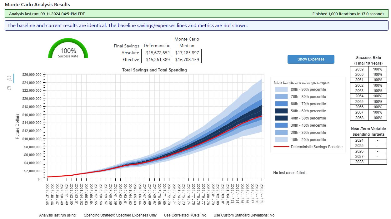
Assets with higher returns will tend to be more volatile than assets with lower returns. If you take a conservative stance relative to the ROR of the assets in your portfolio, then Pralana’s Monte Carlo analysis will depict a narrower range of returns than a portfolio with a more aggressive stance on RORs.
Important Note About Volatility, Correlation, and Rebalancing
When multiple asset classes are modeled with high volatility and no correlation, Pralana’s annual portfolio rebalancing can produce a mathematical effect sometimes called a diversification return or rebalancing bonus. In these situations, the typical (median) Monte Carlo outcome may be noticeably (or dramatically) higher than the deterministic projection, even though the same long-term return assumptions are used.
This result does not indicate an error. It reflects how volatile assets that do not move together can enhance compound growth when regularly rebalanced to target allocations.
If asset classes that behave similarly in real markets (for example, multiple stock-like assets) are modeled as uncorrelated, the Monte Carlo analysis may overstate this effect.
For a detailed explanation, see Appendix 3 – Modeling Market Volatility, Multiple Asset Classes, and Annual Rebalancing in Monte Carlo Simulations.
Historical Analysis
Pralana includes historical inflation rates and market returns for several asset classes—including the S&P 500 Stock Index, 10-year Treasury Bonds, 3-month Treasury Bills, corporate bonds, real estate, and gold—covering the period from 1928 to the present. Using this data, along with any additional historical asset class data you provide, Pralana’s Historical Analysis generates multiple projections that reflect actual historical inflation and market volatility.
Income and expenses tied to inflation (such as Social Security) are adjusted using the historical inflation rates associated with each projection.
Each projection applies a contiguous sequence of historical returns and inflation rates. The first projection begins with the earliest year of available historical data (1928), the next begins in 1929, then 1930, and so on.
For each projection, Pralana requires at least 20 years of historical data at the beginning of the plan. Once the historical sequence reaches the end of the available data, any remaining years in the projection are filled using your specified account-level or asset-class-level rates of return and inflation rates.
This design allows Pralana to generate substantially more historical projections than traditional historical simulators. Many calculators stop generating projections once historical data can no longer span the entire remaining planning horizon, which significantly limits the number of scenarios evaluated.
Pralana instead emphasizes the use of real historical data in the early years of each projection—when market returns have the greatest influence on long-term outcomes—while relying on fixed assumptions only in later years.
A future version of Pralana may allow you to specify the minimum number of historical years required for each projection, rather than using the current fixed value of 20 years.
Historical Rates of Return
To simulate market volatility, Pralana’s Historical Analysis uses annual historical rates of return rather than average returns to determine the annual rate of return (ROR) for each account.
When using Simple Portfolio Modeling, you map each account to one of Pralana’s historical asset classes (or one that you define), and the corresponding historical RORs are used to calculate annual growth in each account.
When using Advanced Portfolio Modeling, you map your asset classes to one of Pralana’s historical asset classes (or one that you define). The historical RORs for those asset classes are then used to determine asset-class growth within each account, based on your asset allocations.
Historical Inflation Rates
All income and expense cash flows which you specified will increase annually based on the general inflation rate will be adjusted using historical inflation rates. Social Security income is always inflation-adjusted and therefore always reflects historical inflation.
Historical Analysis Results
The Historical Analysis chart uses the same color and line conventions as the Monte Carlo chart to ensure consistent interpretation.
The blue solid line shows the scenario’s deterministic projected total savings at the time the analysis was run, and the blue dashed line (when shown) shows deterministic projected expenses at that time. These lines serve as a reference baseline.
The blue shaded bands represent the distribution of projected total savings across all historical sequences, shown as percentiles. Wider bands indicate greater dispersion in outcomes.
If you modify scenario inputs after running the Historical Analysis, green lines may appear. The green solid line shows the current deterministic projected savings based on your updated inputs, and the green dashed line shows current deterministic projected expenses. These lines illustrate how your changes compare to the previously analyzed historical results. To update the shaded bands, rerun the Historical Analysis.
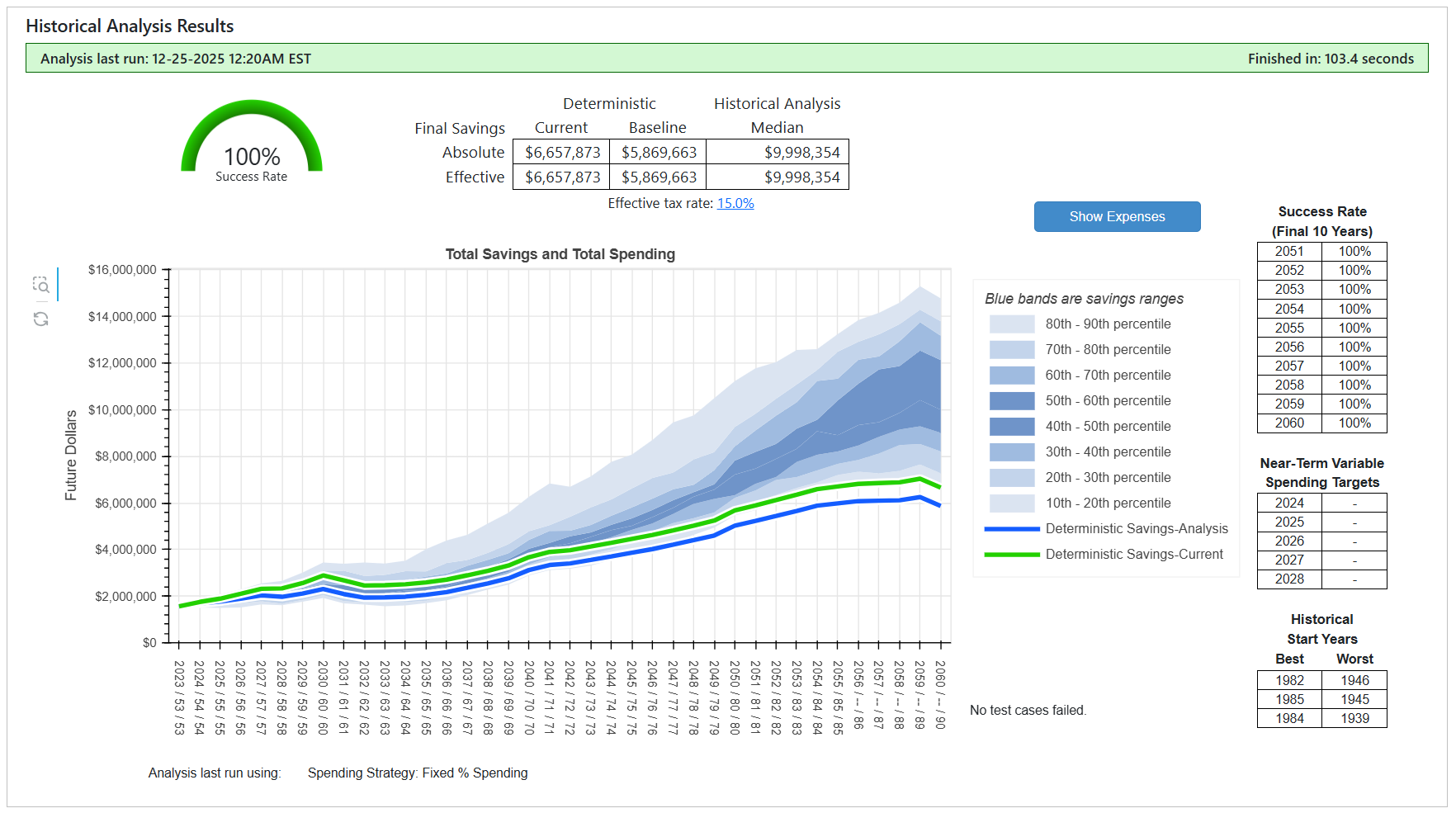
Success Rates and Failed Cases
In the example above, none of the historical test cases ran out of money, resulting in a 100 percent success rate. This is indicated by both the success-rate gauge in the upper left corner of the chart and the final row of the success-rate table to the right. The small table adjacent to the gauge compares final deterministic savings with the median final savings across all historical projections.
Note: In this example the deterministic savings lines are well below medium of the bands because the user’s rates of return are more conservative (lower) than the historical averages for this asset mix.
If any historical test cases fail, the three best and three worst cases are identified in the table beneath the success-rate table. A message is also displayed indicating, on average, how many years before the end of the planning horizon the failed cases ran out of money. These messages are illustrated in the screenshot below. You may explore individual historical sequences in more detail using the Historical Sequence Analysis feature described later in this document.
Historical Rates of Return and Inflation
You can view the historical data in Pralana’s database and add your own historical data via the Historical Rates of Return and Inflation tab on the Analyze > Historical Analysis page.
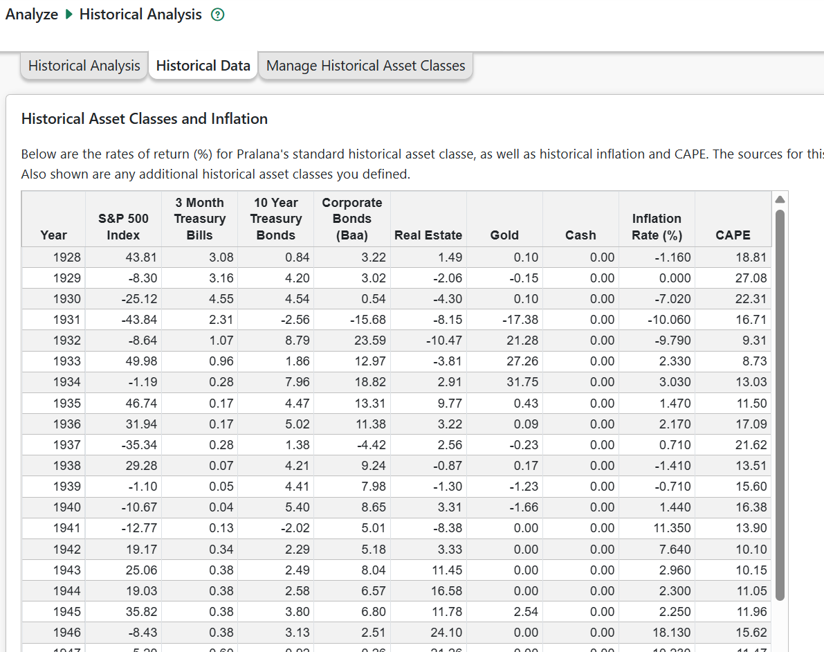
The Historical Data tab shows the nominal rates of return for various asset classes, plus historical inflation rates and CAPE values. These values are provided by Pralana using published data sources identified at More > Resources > General Resources: Data Sources and other Credits. If you have defined custom historical asset classes, this page will display those as well.
Manage Historical Asset Classes
Beyond the historical asset classes and rates of return provided by Pralana, you may create custom historical asset classes. Use the tabs below to map historical asset classes to your accounts or asset classes (depending on which portfolio modeling method you are using) as well as create custom historical asset classes and enter their rates of return.
Map Accounts (or Asset Classes) to Historical Classes
To use the historical asset rates of return in the Historical Analysis, you must specify, or ‘map’, an historical asset class to each of your accounts (if using Simple Portfolio Modeling) or asset classes (if using Advanced Portfolio Modeling) an association between the historical asset classes and your portfolio.
Below is a screenshot of a sample mapping for Simple Portfolio Modeling. The accounts are listed down the left-most column. Because each, you select the historical asset class to use for that account in the Historical Analysis.
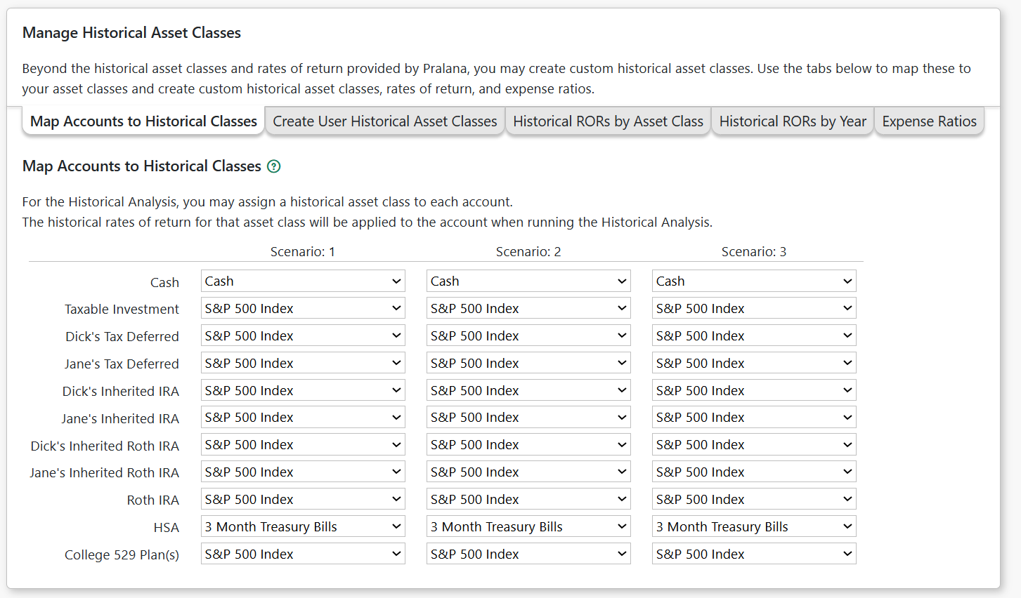
Create Custom Historical Asset Classes
To enter the data for a new class, just enter an Asset Class name in the new row. From your historical data source, copy two columns of data: (years from 1928 through to the current year)
Years: from 1928 through last year (e.g in 2026, copy data from 2028 thru 2025)
RORs: the nominal rate of return for each year
Paste the data into the field labeled: “Paste list of: year, rate of return” and press the tab key or click outside the paste area.
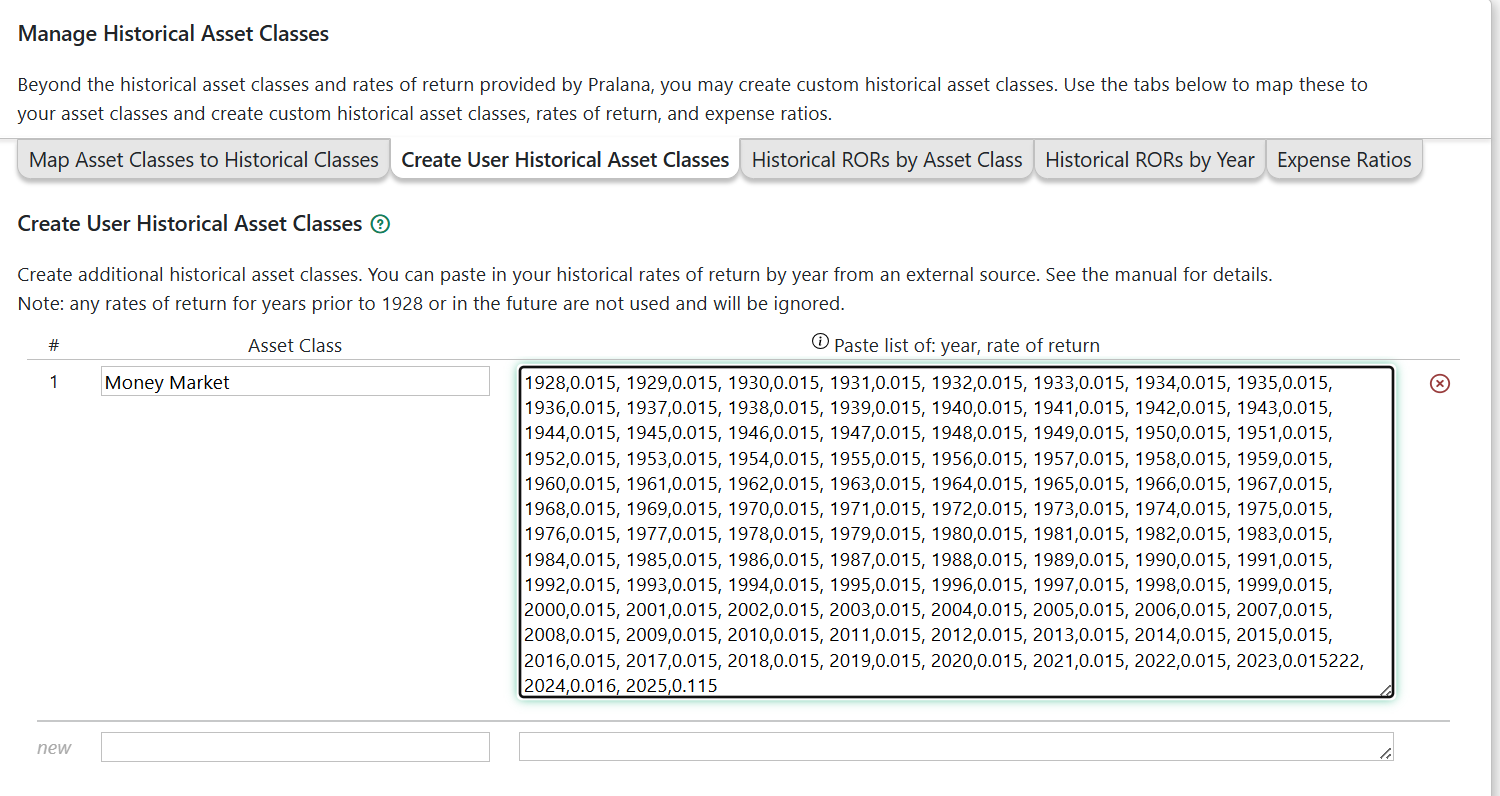

Historical RORs by Asset Class
If you have created one or more user historical asset classes, On this tab you may select the asset class from the dropdown and Pralana will list the years and rates of return, which you may edit.
Historical RORs by Year
Alternatively, you may use this tab to edit the rates of return for all of your custom asset classes for the selected year.
Historical Asset Class Expense Ratios
Published historical rates of return are based on market indexes, which assume no management fees, fund expenses, or trading costs. In practice, investors access these asset classes through mutual funds or ETFs, which overlay annual expenses.
Pralana subtracts the expense ratio you enter from the historical annual return for that asset class. This reduces the nominal rate of return used in the analysis and more closely reflects the returns an investor would have actually realized.
Example: if a historical asset class has a return of 7.0% and you enter an expense ratio of 0.40%, Pralana will use a return of 6.60% for that year.
Monte Carlo and Historical Analysis Results
Both the Analyze > Monte Carlo Analysis and Analyze > Historical Analysis pages share the following features:
Monte Carlo and Historical Analysis results are summarized using percentile bands representing the distribution of outcomes (from the 10th through the 90th percentiles), along with overall success rates.
Expense projections may be overlaid on the graph, allowing you to compare spending against projected savings across analysis methods.
The Monte Carlo and historical analysis results are saved when you click the “Run Monte Carlo (or Historical) Analysis” button, but the green ‘Current’ deterministic analysis results are dynamic.
After running the analysis, if you make any changes that affect those projections, Deterministic Savings and Expenses lines will change to reflect the update scenario projection.
The spending strategy in effect when the analysis was run is identified below the graph.
The “Show (or Hide) Expenses” button will overlay (or hide) the deterministic expense dashed lines and bands showing the range of expenses in the Monte Carlo and historical analyses. The y-axis scale on the right side of the chart show the expense values.
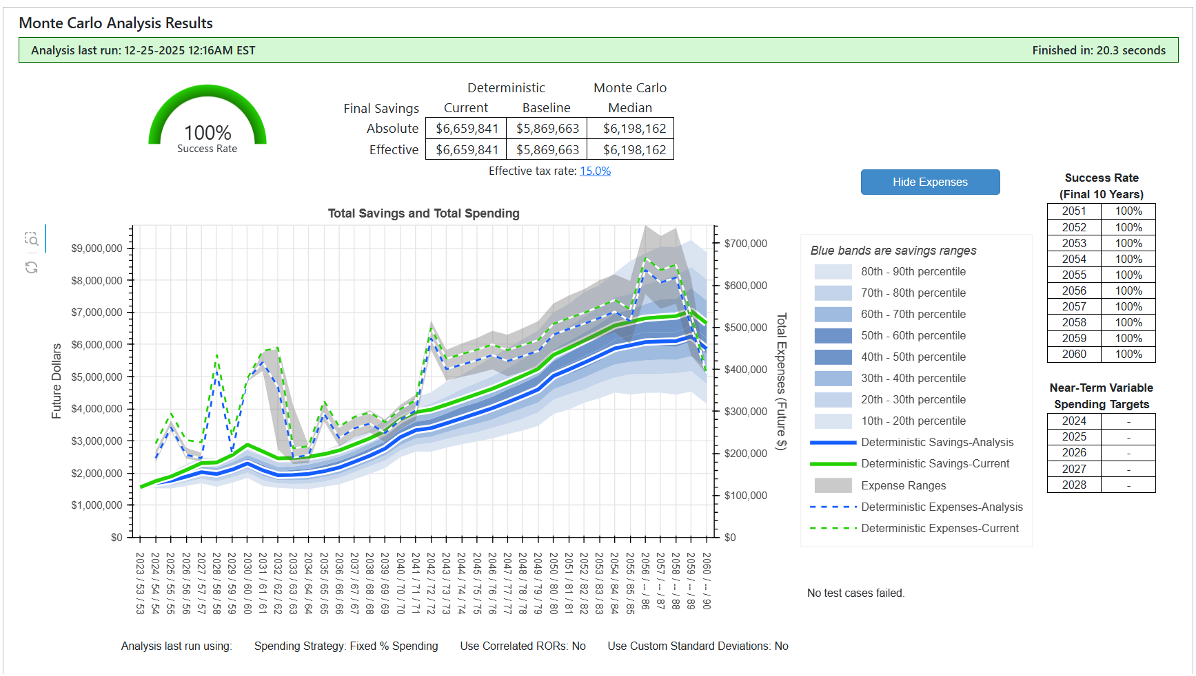
Interpreting the Results
Each Monte Carlo and Historical Analysis generates a very large number of underlying data points over time. Rather than displaying these individually, Pralana summarizes the results by presenting a range of likely outcomes using percentile bands.
The shaded bands represent grouped percentile ranges across all data points generated by the analysis: 10th–20th, 20th–30th, 30th–40th, 40th–60th, 60th–70th, 70th–80th, and 80th–90th percentiles. These bands are stacked in order, with lower percentile ranges shown at the bottom of the chart and higher percentile ranges shown at the top. You may hover over any band to see the specific percentile range it represents.
For example, the 10th–20th percentile band represents outcomes near the lower end of the distribution. Only 10 percent of the data points fall below this band, while the remaining 80 percent fall above it. Taken together, the percentile bands illustrate the distribution of plausible outcomes produced by market volatility.
In the example shown, final savings vary widely—from approximately $4 million to $9 million—highlighting the significant impact that market volatility can have on long-term portfolio performance. For reference, the deterministic projection captured at the time the analysis was run is overlaid on the chart (solid blue line) and typically lies near the median (50th percentile) of the distribution.
Total Spending
The Total Spending illustration shows how projected spending varies over time under deterministic, Monte Carlo, or Historical Analysis. Total spending is plotted against the right-hand vertical axis of the graph.
The dashed blue line represents total spending from the deterministic projection when the analysis was run. The shaded envelope around that line represents the range of total spending produced by the Monte Carlo or Historical Analysis. The lower edge of the envelope corresponds to the 10th percentile of results, and the upper edge corresponds to the 90th percentile.
Total spending expands into a range of possible outcomes under Monte Carlo or Historical Analysis for two primary reasons:
Tax variation:
Taxes vary with portfolio performance. When portfolio returns are higher (for example, in the 60th–90th percentile outcomes), taxes tend to be higher due to larger required minimum distributions and higher taxable investment income. When portfolio returns are lower, taxes tend to be lower for the same reasons. An internal analysis confirms a strong correlation—approximately 95 percent—between total savings and total expenses driven by these tax effects.
Spending strategy variation:
Some spending strategies explicitly link spending levels to portfolio performance. For example, under a fixed-percentage spending strategy, higher portfolio values allow for higher spending, while lower portfolio values require reduced spending. This effect does not apply when using the Specified Expenses Only or Consumption Smoothing strategies, where spending is not directly tied to portfolio performance.
Why Do Expenses Drop Dramatically in the Final Year?
You may see a noticeable reduction in expenses in the final year of the projection. This occurs because Pralana models the final year as a partial year of income and expenses, based on the birthday of the last-surviving spouse.
Historical Sequence Analysis
The Historical Sequence Analysis lets you test the long-term impact of one specific historical sequence of returns and inflation for your selected asset classes, income and expenses.

Pralana will recalculate the scenario’s deterministic savings and expenses and show them on the chart with green lines.
Except for the RORs and inflation rates, all other parameters, income and expense details are identical to those of the normal deterministic projection.
Best practice is to run the Historical Analysis prior to enabling the Historical Sequence Analysis to ensure that the blue projection lines (Deterministic-Analysis) are based on all your current inputs. Then, enable the Historical Sequence Analysis. By doing this, the only differences between the deterministic-analysis projections (the blue lines) and the deterministic-savings (green lines) are the inflation and rate of return sequences.
Click the ‘View Historical Sequence’ button to see how the historical rates of return and inflation rates are applied to your scenario’s years. The historical data for the year you entered as the “Historical Sequence Analysis Start Year” will map to the scenario’s first year and with subsequent years of historical data applied to subsequent scenario years.
Variable Spending Strategies
A ‘deterministic’ analysis of your plan with specific income, expenses, and portfolio performance is a great way to evaluate its fundamental viability and compare alternatives. ‘Deterministic’ means the scenario projection are calculated, for all years, using your specified inputs.
In the real world, though, if your portfolio was underperforming your expectations, you probably adjust your spending over time, based on your portfolio’s performance to avoid outliving your money. Pralana supports these eight strategies for making spending adjustments:
Consumption Smoothing
Constant Spending
Fixed % Spending
Fixed % Spending with Floor and Ceiling
Guyton-Klinger Rules
Target % Adjustment
Actuarial
CAPE Rules
Spending strategy selection and inputs are on the Analyze > Spending Strategies page.
Six of these strategies are described in a paper by Wade D. Pfau (Professor of Retirement Income at The American College, Bryn Mawr, PA) entitled Making Sense Out of Variable Spending Strategies for Retirees. All these spending strategies can be applied to deterministic projections as well as Monte Carlo and Historical Analyses.
A 9th strategy, CAPE Rules (Cyclically Adjusted Price Earnings ratio-related rules), is applicable only during historical analyses and is, therefore, enabled on the Analyze > Historical Analysis page.
You can read more on each spending strategy in subsequent sections.
The Audits tab provides insight into the calculation of the variable spending amount for most strategies.
Important Spending Strategy Concepts
Specified Expenses Only (default): scenario projections are based strictly on your inputs provided on the Get Started, Financial Assets, Income and Expenses pages.
Consumption Smoothing: scenario projections are calculated the same as for Specified Expenses Only plus Pralana adds an amount for “consumption-smoothed expenses” generated by consumption smoothing algorithm in all plan years. This is a single calculated amount adjusted annually for inflation.
All other strategies: scenario projections are calculated the same as Specified Expenses Only except as follows:
These strategies apply only after retirement. In single plans, they affect spending in the retirement year; in married plans, they affect spending in the year when both spouses have retired.
Your non-essential expenses are replaced by the strategy’s calculated ‘variable expense’. Non-essential expenses include Phased and Miscellaneous Expenses that are designated ‘non-essential’ as well as non-QCD Charitable contributions. (Pralana considers your QCD’s to be essential).
Essential expenses are never changed. Essential expenses include expenses for Property, Rental, Children, Healthcare and Life Insurance Expenses pages, QCD expenses from the Charity page, and essential expenses from the Phased and Miscellaneous Expenses pages.
The Spending Rate parameter: Many of these strategies use a ‘spending rate’ which refers to your non-essential spending rate, not your overall spending rate. For users of Pralana Gold, you will recognize this as being the same as the Pralana Gold approach. Note: For your information, this approach may be enhanced in an upcoming update such that the Spending Rate parameter will optionally refer to your overall spending rate, including essential and non-essential spending plus all taxes. The revised implementation will be more consistent with the terminology used by Wade Pfau.
Pralana’s tabular projections, charts and other representations of your scenario projections will always reflect the active spending strategy.
Pralana’s Monte Carlo Analysis and Historical Analysis will run using the active spending strategy as will the optimization features for Roth conversions, Social Security Start Ages, Withdrawal Priorities, and Earliest Safe Retirement.
Consumption Smoothing
Pralana’s consumption smoothing provides three ‘solution types’ which allow you to specify a goal and Pralana will calculate the consumption-smoothed spending (CSS) amount to reach that goal:
Deterministic: You specify your goal for the scenario’s final effective savings, in today’s dollars.
Monte Carlo and Historical: You specify a goal success rate, e.g. 75% or 90%.
Each solution type requires iteration. Pralana will iteratively guess a spending amount, run the calculations, adjust the guess and recalculate until the result is within a small tolerance of your goal.
When the analysis is complete, the summary results will be shown along with a chart showing the spending amounts evaluated and the result (savings or success rate) each yielded.
Important notes about Consumption Smoothing:
The calculated spending amount may be positive or negative. Positive amounts mean you can spend more than your specified expenses and achieve your goal. Negative amounts mean you need to reduce your spending to achieve your goal.
The calculated CSS amount (inflated) will be included as an expense in all scenario years, with two possible adjustments:
In the years before you retire (or the 2nd spouse to retire, for two-person plans), Pralana will reduce the CSS amount $1-for-$1 by the amount of your employment contributions to retirement plans (tax-deferred, Roth and defined benefit plans). Note: Pralana uses the retirement date(s) you provide to make this determination. If you continue to work and make retirement contributions from wages after your retirement date, Pralana will not reduce the CSS amount in those years.
For two-person plans, Pralana assumes the consumption smoothing amount may decrease after the death of the first spouse. Pralana uses the “% Reduction for Survivor” you specify for Phased Expenses to calculate this decrease.
In rare cases, no solution may be found that achieves the goal. For the Deterministic solution, particularly, a very small change (a few cents) in the consumption-smoothed spending amount may increase a taxable withdrawal just enough to trigger a tax or IRMAA ‘cliff’ in one or more years. Compounded over many years, the jump in tax expense may lead to a sizable reduction in final savings.
Here are some resources where you can learn more about consumption smoothing:
A book entitled “Spend ‘til the End” by Laurence Kotlikoff and Scott Burns.
A Forbes article by Wade Pfau entitled Lifetime Finance: An Alternative for a Lifetime Financial Plan (Lifecycle Finance: An Alternative For A Lifetime Financial Plan (forbes.com)
An alternative and equally important use of Pralana’s consumption smoothing capability is to gain insight into the amount of margin that exists in your plan: the Calculated Consumption-Smoothed Spending field is the amount by which your annual spending can be increased without you running out of money in your expected lifetime.
The Deterministic Algorithm
Here is a screenshot of a deterministic consumption smoothing example:
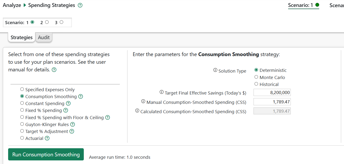
At the bottom of the page is a graph showing the consumption-smoothed spending amounts that were evaluated.
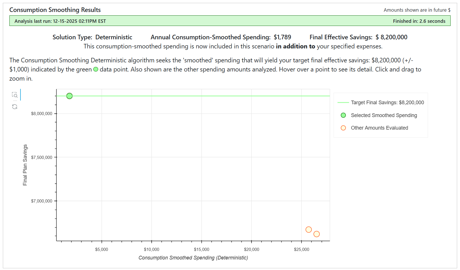
Please note the Manual Consumption-Smoothed Spending (CSS) field, located just above the Calculated CSS field. You can manually enter a value in this field (in today’s dollars) and it will override the calculated CSS value.
This consumption-smoothed spending amounts are shown in the Expense Statement.
Monte Carlo and Historical Solution Methods
Pralana can run Monte Carlo or historical analyses iteratively, varying the CSS amount in each run, to find the amount that yields a probability of success near the target you specify. (i.e., the percentage of test cases that resulted in a positive final effective savings).
After selecting the solution type and specifying your target savings or success rate, click the “Run Consumption Smoothing” button to initiate the calculations. The Monte Carlo and historical methods will always take longer to execute than the deterministic analysis because there is much more computation being done.
When the process is completed, the Manual and Calculated Consumption-Smoothed Spending field will contain the calculated CSS amount in today’s dollars. You may override the calculated value by making an entry into the Manual Consumption-Smoothed Spending field. Pralana will include the CSS amount as an annual inflation-adjusted expense as long as the Consumption Smoothing strategy is active.
Also, you add the CSS amount on the Phased expenses page and then disable Consumption Smoothing.
Example
Using the screenshot below as an example, Pralana computed CSS at $30,278. As described above, in the years prior to retirement, Pralana reduced the CSS amount by the amount of employment contributions to savings. In this example, full-time employment ends in the year 2035. Prior to 2035, the CSS amount is reduced to $17,778 in Today’s $.
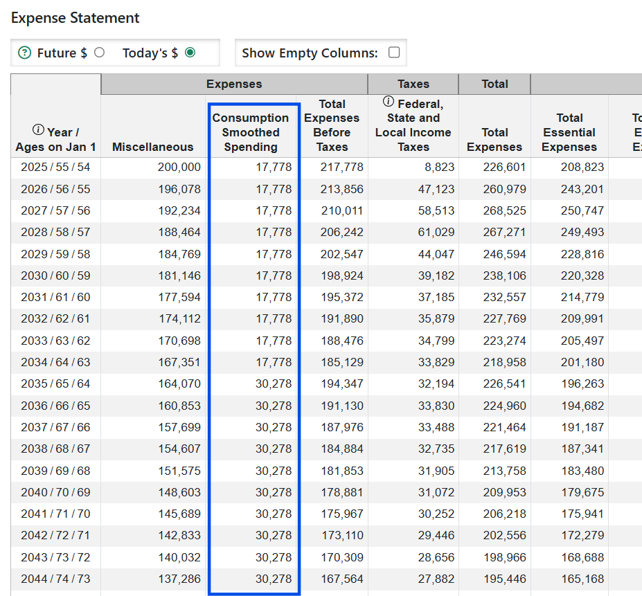
Constant Spending Method
Variable expense at the start of retirement is established using the fixed-percentage method. Thereafter, spending is adjusted annually based solely on inflation to maintain a constant, inflation-adjusted level of non-essential spending.
Because spending does not automatically adjust downward in response to poor portfolio performance, this method has the potential to fully deplete savings over time.
Fixed Percentage Spending Method
Variable expense in each year of retirement is calculated as a constant percentage of remaining savings. Because spending is directly tied to portfolio value, annual spending will rise and fall with market performance.
Unless essential spending overwhelms available resources, this approach prevents complete depletion of savings by automatically reducing non-essential spending as portfolio balances decline.
Fixed Percentage Spending with Floor and Ceiling Method
This method begins with the fixed-percentage approach but imposes limits on how much variable expense can increase or decrease over time. A ceiling prevents spending from rising above a specified percentage above the real (inflation-adjusted) level of first-year retirement spending, and a floor prevents spending from falling more than a specified percentage below that level.
The intent is to smooth year-to-year spending fluctuations while still allowing spending to respond to portfolio performance. When you select this method, Pralana provides input fields for the initial spending rate as well as the ceiling and floor percentages.
Guyton-Klinger Spending Method
With this method, initial variable expense is established using the fixed-percentage approach. Thereafter, variable expense is adjusted based on inflation, portfolio performance, and deviations from the initial spending level, following the Guyton-Klinger decision rules.
Variable expense is adjusted annually for inflation unless the portfolio experienced a negative return in the prior year and the current spending rate exceeds the initial spending rate. Variable expense is increased by 10 percent when the current spending rate falls at least 20 percent below its initial level (the prosperity rule). During the first 15 years of retirement, variable expense is reduced by 10 percent whenever the current spending rate exceeds the initial rate by at least 20 percent (the capital preservation rule).
This strategy can result in higher initial spending, followed by reductions if portfolio performance deteriorates. When you select this method, Pralana provides an input field to specify the initial spending percentage.
Target Percentage Adjustment Spending Method
This method establishes a target savings trajectory based on total savings at the start of retirement and a specified annual spending percentage. Initial variable expense is set so that projected savings follow this target path.
In subsequent years, variable expense is adjusted for inflation only when projected savings exceed the target trajectory. If projected savings fall below the target, variable expense is not increased for inflation in that year. This approach allows spending to adapt gradually to portfolio performance while attempting to maintain a desired savings profile.
Actuarial Spending Method
The actuarial spending method calculates sustainable annual variable expense based on remaining portfolio balance, remaining longevity, and expected portfolio returns. You may also specify a desired legacy value, expressed in today’s dollars, for the final savings balance. This legacy value is inflated using the general inflation assumption to determine the desired future amount.
The actuarial algorithm currently uses prior-year savings and expenses to calculate each year’s variable expense. As a result, final savings will generally be close to—but not exactly equal to—the desired inflated legacy value. A future enhancement may use iterative tax calculations to more precisely target the specified legacy amount.
CAPE Spending Strategy
The CAPE spending strategy calculates variable expense based on remaining portfolio balance, a user-specified base withdrawal rate, the Cyclically Adjusted Earnings Yield (CAEY), and a user-specified multiplier. This method tends to produce smoother spending patterns than approaches based solely on current portfolio value.
CAPE-based spending is only applicable during Historical Analysis, since the CAPE and CAEY are derived from historical price-to-earnings data. Deterministic and Monte Carlo analyses do not use historical CAPE values; therefore, if the CAPE strategy is selected for those analyses, Pralana defaults to using specified expenses only.
Two parameters control this method: a base withdrawal rate and a multiplier applied to the CAEY. The variable withdrawal rate is calculated as the prior year’s portfolio value multiplied by the sum of these two components, which helps moderate year-to-year fluctuations.
The CAPE spending strategy is used only in Historical Analysis and is not applied to other analyses or optimization features, including Roth conversion optimization.
Final Notes on Variable Spending Strategies
Total spending includes income taxes in addition to essential expenses and the variable expenses generated by the selected strategy. In retirement, taxes can become a significant component of total spending—particularly after required minimum distributions begin—and this can increase the variability and dispersion of projected spending outcomes.
Roth Conversions
Pralana allows you to model Roth conversions of your (and, if married, your spouse’s) tax-deferred savings into a Roth IRA. Pre-tax conversion amounts are taxable as ordinary income. If the source tax-deferred account includes after-tax contributions, the conversion will include a pro-rated portion of after-tax funds in accordance with IRS pro-rata rules.
The radio buttons at the top of the Roth Conversions page allow you to specify the active scenario and enable or disable Roth conversions.
Pralana gives you a high degree of control over both the timing and size of conversions by allowing you to specify:
the years in which conversions may occur,
the source tax-deferred account(s),
the conversion limiting factors including marginal ordinary income tax bracket, LTCG tax bracket, IRMAA bracket and FPL (Federal Poverty Level) multiple,
specific conversion amounts you may specify
The Effect of Asset Allocations on the Evaluation of Roth Conversions
Before evaluating Roth conversions, it is important to understand how asset allocation can influence the results.
Unless you are using account-level asset location mode with identical allocations in all account types, moving money between account types (such as converting from tax-deferred to Roth) will change your overall portfolio allocation. This, in turn, changes:
Expected returns
Risk level
Taxes
Long-term outcomes
When this occurs, it becomes difficult to isolate the true financial benefit of the Roth conversion itself.
Example
Suppose you have:
$1,000,000 in a tax-deferred account invested 100% in bonds earning 2.5%
$750,000 in a taxable account invested 100% in stocks earning 5%
$500,000 in a Roth account invested 100% in stocks earning 5%
The total portfolio is 56% stocks and earns an overall return of approximately 3.9%.
Now suppose you convert $500,000 from the tax-deferred account to the Roth account.
After the conversion:
The tax-deferred account holds $500,000 in bonds
The Roth account holds $1,000,000 in stocks
The taxable account remains unchanged
The overall portfolio allocation increases to 78% stocks, and the expected return rises to approximately 4.4%.
The Roth conversion now appears highly favorable — but much of the improvement is due to the increased stock allocation, not the tax benefit of the conversion itself. The portfolio has become more aggressive, and risk has increased.
Why This Matters
If you use account-level allocation mode while holding different allocations across account types, Roth conversions will also cause asset allocation shifts.
This creates a “bad experiment”. You are measuring the combined effect of:
A Roth conversion, and
A shift toward a different asset allocation.
The result may exaggerate the apparent benefit of Roth conversions. This is not a Pralana issue — it is simply mathematics.
Best Practices
There are two sound approaches:
1) Account-Level Allocation with Mirrored Allocations (Mode 1)
Use the same asset allocation in all account types. This preserves your overall allocation before and after conversions and allows a clean comparison. Pralana allows up to four allocation changes over time, so you can still model a glide path. This approach is often considered the “gold standard” for evaluating Roth conversions.
2) Overall Allocation Mode (Mode 2)
Use Pralana’s overall allocation mode (sometimes called “tax-efficient asset location”). This maintains your target overall asset allocation automatically while allowing you to place bonds and stocks in tax-efficient locations.
This approach may increase expected returns by shifting higher-growth assets into Roth accounts — but the higher return comes from higher effective risk.
You can verify this by running poor historical sequences (e.g., 1966) and observing how results differ between modes.
Key Insight
When you load tax-deferred accounts with bonds and Roth accounts with stocks, you are effectively increasing your exposure to equities. The government shares in the risk of tax-deferred assets, but Roth assets are entirely yours.
The additional return often observed under tax-efficient asset location is compensation for taking additional risk — not “free money.”
Pralana gives you the tools to test this yourself.
Practical Tip
If you prefer holding different allocations in different accounts, a useful approach is to:
Evaluate Roth conversions under mirrored allocations (Mode 1), and
Evaluate again under overall allocation mode (Mode 2),
Then choose a conversion amount somewhere between the two outcomes.
Roth Conversion Parameters
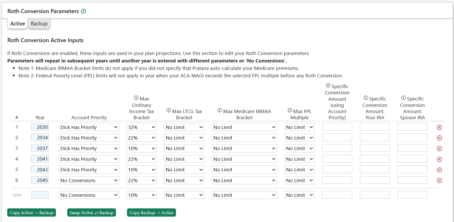
Active Parameters
Use this page to enter the parameters to control Pralana’s Roth conversion modeling.
If you wish to use the same parameters for multiple years, you do not need to replicate the rows. Enter the first year and the associated parameters. Pralana will use those parameters for all subsequent years until parameters for a later year are defined.
For example, to use a set of parameters for five years starting in 2030, enter those parameters for 2030. Then create a row for 2035 and specify Account Priority = “No Conversions”.
Tip: You should always enter the year when you want Roth conversions to end and specify “No Conversions” in the account priority field. If you do not, Pralana will evaluate conversions through the final year of your scenario whenever you update inputs. This can significantly slow page response time, analyses, and optimization runs.
Year: This is the start year for Roth conversions using the parameters on this row. As noted above, these parameters will be applied in each subsequent year until a later conversion year is defined or the end of the scenario.
Account Priority: Pralana can model Roth conversions from one or both spouse’s taxed deferred accounts. Options are shown in the drop-down.
If you specify “No Conversions”, Pralana will not perform conversions in that year, or thereafter (unless a later conversion year is defined).
If you specify “proportional”, conversions are split between accounts in proportion to their relative balances.
Max Ordinary Income Tax Bracket: This is the primary control that determines the annual Roth conversion amount. Pralana calculates the difference between:
The top of the selected ordinary income tax bracket, and
Your projected ordinary taxable income, before Roth conversions.
That difference becomes the maximum Roth conversion amount for the year — unless another limiter (IRMAA, LTCG, FPL) limit is reached first.
Max LTCG Bracket: Roth conversions increase your Federal AGI, which can increase long-term capital gains taxes. This control limits conversions to keep your income within a selected LTCG bracket. Select “No Limit” if you do not want LTCG brackets to restrict conversions.
Max Medicare IRMAA Bracket: Roth conversions increase Medicare MAGI, which may increase Medicare Part B and Part D premiums due to IRMAA rules (with a two-year lookback). If you have enabled automatic Medicare premium modeling on the Healthcare Expenses page, Pralana will calculate these premium changes.
This control allows you to limit annual Roth conversions so that your MAGI does not exceed a selected IRMAA threshold. Thresholds are shown in today’s dollars and are inflation-adjusted annually. Select “No Limit” if you do not wish to limit conversions based on IRMAA.
Max FPL Multiple: ACA subsidies depend on your ACA MAGI relative to the Federal Poverty Level (FPL). Roth conversions increase MAGI and may reduce or eliminate ACA premium subsidies.
This control allows you to limit conversions so that your MAGI does not exceed a selected multiple of the FPL. Available breakpoints correspond to ACA rules (e.g., 1.5×, 2×, 2.5×, 3×, 4× FPL). Select “No Limit” if ACA subsidies do not apply to you or if you do not want to restrict conversions based on FPL multiples.
Specific Conversion Amounts: These fields allow you to override Pralana’s automatic bracket-based conversion calculation by specifying fixed pre-tax Roth conversion amounts. You should enter amounts in Today’s $. The amounts will be inflation-adjusted using your general inflation rate. If the source accounts include after-tax balances, a pro-rated after-tax amount will also be converted.
Using Account Priority: If an amount is entered here, Pralana will convert that amount using the selected Account Priority setting for the year. “Proportional” splits the amount between both IRAs based on relative balances. Priority settings determine which IRA is used first when applicable. If entered, this field overrides the individual IRA amount fields below.
Your IRA: If an amount is entered here, that amount will be converted from your IRA only, regardless of Account Priority.
Spouse IRA: If an amount is entered here, that amount will be converted from your spouse’s IRA only, regardless of Account Priority.
Active / Backup Buttons: Pralana provides three buttons to allow you to copy or swap the active and backup Roth conversion parameters. Changes that would overwrite the active parameters require you to confirm the action.
Backup Parameters
This page shows the ‘backup’ Roth conversion parameters. These are a copy of your active parameters and provide a way for you to change the active parameters to test various conversion strategies and, at any time, restore your original parameters. The Backup Parameters are updated whenever you:
You run Optimize Roth Conversions, or
You click the ‘Copy Active → Backup’ or ‘ Swap Active ⇄ Backup’ buttons on the Active Parameters page.
Roth Conversion Results
This page contains a tabular projection showing Pralana Roth conversion calculation results.
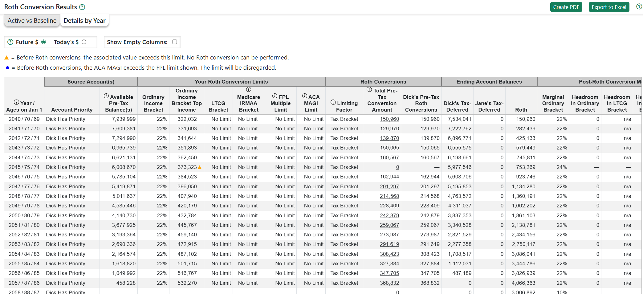
Here are some observations on the example above:
Conversions begin in the year 2040.
From year 2040 onward, the 22% tax bracket is the limiting factor on how much is converted each year, and on the right you can see that the Roth conversions completely fill the bracket (since there is no remaining headroom in the ordinary bracket).
In 2045, no conversion is done because ordinary income exceeds the top of the 22% bracket before any Roth conversions are done.
You may click on an amount in the ‘Total Pre-Tax Conversion Amount’ column to pop-up the associated Metric MRI showing details of how that amount was calculated.
Optimize Roth Conversions
Pralana’s Roth conversion optimization algorithm evaluates many Roth conversion strategies to identify the strategy that yields the highest final effective savings.
A conversion strategy is defined as a specific set of conversion parameters — that is, the ordinary income tax brackets applied across the Roth conversion years. For example, a strategy might use the 10% bracket for several years and the 22% bracket thereafter.
The optimization process uses your specified LTCG bracket, IRMAA bracket and FPL Multiple settings. However, it disregards any user-specified conversion amounts.
See “Roth conversion FAQs” below for an explanation of why it is not feasible for Pralana to evaluate all possible conversion strategies.
A 3-pass algorithm is used to determine the optimum marginal brackets for every year in the conversion period.
Before starting, the optimizer will copy your Active Parameters to Backup Parameters so that they may be restored if desired.
First pass: The algorithm iterates through all ordinary income tax brackets and evaluates strategies that apply the same bracket to all conversion years. It determines which bracket produces the highest final effective savings.
Second pass: The algorithm begins with the best overall bracket identified in the first pass and applies it to all years. It then seeks improvements on a year-by-year basis. It starts with year 1 and tests all brackets for a possible improvement in the final savings balance while all future years are using the best overall bracket established in the first pass. It then modifies the bracket for year 1 with the bracket yielding the best long-term result. Then it tests all brackets in year 2 for a possible improvement in the final savings balance while all future years are using the best overall bracket established in the first pass. It then modifies the bracket for year 2 with the bracket yielding the best long-term result. This process is repeated for all remaining years in the modeling period.
Third pass: The process is repeated using the results of the second pass as the starting point, allowing one final refinement of the marginal tax bracket in each year.
The algorithm also includes your current/active Roth conversion strategy.
Preserve User-Specified Roth Conversion Amounts
If you have entered specific Roth conversion amounts in your strategy, Pralana will, by default, ignore and remove those amounts during optimization.

Check this box if you want Pralana to retain and apply your specified conversion amounts in the applicable years while optimizing the remaining conversion strategy.
Roth Conversion Results
Below is a screenshot showing a sample of the optimization results. The table displays the number of conversion strategies evaluated and other relevant information. The chart plots the final effective savings for each evaluated strategy. Strategies (data points) are sorted from best to worst (by final effective savings) from left to right. Hover over a point to view the associated conversion years and ordinary income tax brackets.
It is common and expected for multiple strategies to produce the same final result. This can occur, for example, when your tax-deferred accounts are fully converted resulting in a zero balance. In subsequent years, all variations of the ordinary income tax bracket will produce identical results because no further conversions can be performed.
If the algorithm identifies a conversion strategy (or strategies) that produces higher final effective savings than your current strategy, Pralana updates (overwrites) your active Roth conversion parameters with those of the optimal strategy.
If the algorithm’s best strategy produces the same final effective savings as your current strategy, Pralana will display an alert and will not change your parameters. This typically occurs when you have previously run the optimizer and your current strategy is already optimal.
It is also possible to manually create a strategy that produces higher final savings than any of the optimizer-created strategies. If this occurs, the optimizer will alert you and will not alter your strategy.
If you choose not to use the optimized parameters, you may click the “Copy Backup → Active” button on the Active Parameters page to restore your pre-optimization parameters.
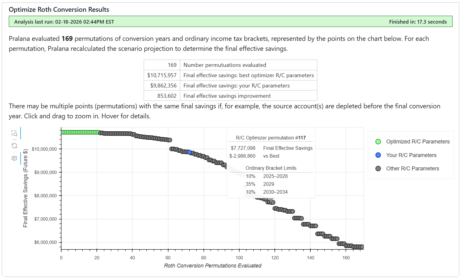
Current vs Baseline
This page is the same as the Review > Graphical Projections > Current vs Baseline page and is provided here as a convenience to see the impact of changes to Roth conversion parameters on the scenario projections.
A Note on IRMAA Limitations on Roth Conversions
Your Medicare premiums in the current year are a function of the relationship between your Medicare MAGI from the 2nd prior year and IRMAA brackets for the current year. Therefore, when Pralana computes your IRMAA-limited Roth conversions, it does so by limiting the conversions (and your MAGI) in the current year so that it does not exceed the specified IRMAA limit two years in the future.
Taxes on Roth conversions
Pralana does not reduce the conversion amount to withhold funds to pay for tax triggered by the conversion. The pre-tax amount of the conversion is included in taxable income in the conversion year which is used to calculate estimated federal, state and local tax payments for the year. Estimated tax payments are included in expenses and net cash flow.
Roth conversion FAQs
Assume 25 conversion years. There are 8 ordinary income brackets for each year.
The number of permutations is 8 to the 25th power = 37,778,931,862,957,161,709,568.
To evaluate the final plan savings for each permutation, Pralana needs to do a scenario recalculation.
If the scenario recalculation takes 0.1 seconds, evaluating all permutations would take 119,796,207,074,318 years.
If we could speed that up 1,000-fold. That would be only 120 billion years.
Ideally, the Optimizer would evaluate all permutations of all inputs for each R/C year: 8 tax brackets, 2 account withdrawal priorities, 3 LTCG brackets, 6 IRMAA brackets, and 6 FPL brackets = 8 * 2 * 3 * 6 * 6 = 1,728 permutations per scenario year.
Calculating 1,728 ^ 25 permutations would take 2.75 x 10^72 years, much longer than the age of the universe.
Optimize Social Security Start Age
If your Social Security benefits have not already started, Pralana will conduct an analysis to determine the ages at which you and your spouse (if applicable) should start taking benefits (on your own records, respectively) to maximize your effective savings at the end of the modeling period. The only variables this analysis considers are your Social Security benefit start ages and it does include spousal benefits in its calculations; it assumes you retire from full-time employment as described on the Build > Get Started > Scenario Assumptions page. The analysis Pralana performs during this process is considerably more involved than just determining the start ages that result in the largest long-term SS income; instead, it examines the long-term effects of this income on your savings, taxes, and survivor scenarios (i.e., what-if scenarios you may have set up to investigate the premature death of you or your spouse) to provide you with the best overall solution which, in turn, will enable you to maximize your standard of living. Further, since the mathematically best solution may be only slightly better than some other solutions, Pralana examines the set of possible solutions associated with all start dates and identifies the subset of these that are almost as good as the best one. Through the “Sub-Optimum Selection Threshold” field, you can control the range of alternate solutions that Pralana will identify as viable alternate solutions. The value you enter in this field is used by Pralana as a threshold and if the long-term results of other solutions are above the specified percentage of the best solution, they will be highlighted.
Clicking the Optimize Social Security Start Ages button on the Analyze > Optimize Social Security Start Age page will trigger Pralana to calculate the optimum ages for you and your spouse (if applicable) to begin taking Social Security benefits. The result will be reflected as a dark green dot in the matrix diagram. Pralana will also calculate slightly sub-optimum ages, based on the Sub-Optimum Selection Threshold percentage that you specify, and these ages will be reflected as lighter green dots in the matrix. In the immediate vicinity of the dark optimum dark green dot, the lighter green dots will be placed with one month granularity and slightly farther away from the optimum position the light green dots will be placed with three months granularity. If you wish to see the optimization results in greater detail, you can zoom in. To do this, click the Zoom icon on the left side of the matrix to enable the Zoom function (a vertical bar will appear on the right side of the icon when Zoom is enabled) and then use your cursor to draw a box around the area of interest (point to one corner of the desired box, click and hold, then drag to another corner, then unclick) and that area will be expanded. If you want to zoom in even closer, just use the cursor to draw another box around the area of interest and it will be expanded further. At any point, you can just hover your cursor over a dot and you will get a pop-up that provides details on the related start ages and a comparison between the final savings balance that would result from using these start ages versus the optimum start ages. To return to the original zoom level, just click the Reset icon next to the Zoom icon.
If either your or your spouse’s benefits have already started, optimization of the start age for that partner is moot and will not be performed. In that case, the matrix will contain only one column or one row which depicts the optional start ages for the partner whose benefits have not yet started.
Some additional calculated outputs are provided in the box just above the optimized results matrix. These depict your final effective savings for the Social Security start ages currently specified on the Build > Income > Social Security Income page and the what-if final effective savings if those inputs were changed to the optimized values. To incorporate the insights you gained here into your plan, you will need to go to the Build > Income > Social Security Income page and revise the Social Security start ages specified previously. Note that a shortcut is provided: just click the blue button labeled “Edit Social Security Inputs” and it will take you directly to the relevant page.
Here are some screenshots. The first one shows the page immediately after completing an optimization.
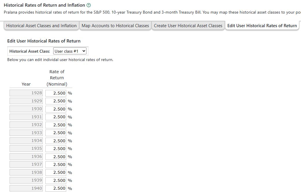
The shot below shows a portion of the matrix after zooming in, with the cursor over one particular result. You can then see the corresponding start ages, the what-if final savings value and how much it differs from the optimum start ages associated with the dark green dot.
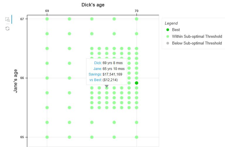
Optimize Withdrawal Priorities
We will begin this section with a quick review of how Pralana manages your Cash Account. The cash account is central to all cash flow in Pralana. All positive cash flows are treated as deposits to the Cash Account and all negative cash flows are treated as withdrawals from the Cash Account; however, it has user-specified minimum (floor) and maximum (ceiling) levels. An overflow condition occurs when those deposits would cause the balance to exceed the ceiling. When that happens, the excess money is withdrawn from the Cash Account and deposited in the Taxable Investment Account. An underflow condition occurs when negative cash flows would cause the balance to go beneath the floor. When that happens, Pralana will seek another source of funds to cover the spending deficit and will refer to the user-specified settings in the Withdrawal Priority Table on the Build > Financial Assets > Management > Account Withdrawal Priority page to make subsequent account withdrawals. In a plan with no deficit spending, the account withdrawal priority is irrelevant and meaningless.
In plans with deficit spending, Pralana’s Optimize Withdrawal Priorities (OWP) algorithm seeks to identify the best account withdrawal priorities to cover deficit spending and maximize final effective savings. The analysis calculates final effective savings for up to 625 combinations of withdrawal priorities based on time periods defined by the distinct years in this list: scenario start year, first retirement year, first RMD year, and the scenario end year.
‘First retirement year’ means the year earlier of the retirement years in two-person plans.
‘First RMD year’ means the earlier of the first year of requirement minimum distributions in two-person plans.
First retirement year and/or first RMD year are disregarded if they fall before the scenario start year or after the scenario end year.
The OWP algorithm’s time periods are the gaps between these two, three or four distinct years.
For example, many users will have three time periods: 1) scenario start to first retirement, 2) first retirement to first RMD, and 3) first RMD to scenario end. Others may have two time periods if the first retirement year and first RMD year are the same year: 1) scenario start to first retirement/first RMD and 2) first retirement/first RMD to scenario end. Likewise, users may have two time periods if, for example, the first retirement year is prior to the scenario start. Finally, some users may have just one time period if they are already retired and have started RMDs at the start of the modeling period.
If there are three time periods, OWP will optimize the second and third periods and assume the user-provided withdrawal priority in the first time period. If there are one or two time periods, OWP will optimize each period.
For each optimization time period, OWP will calculate the scenario’s final effective savings using 24 permutations of withdrawal order, plus the Proportional withdrawal option, from these four accounts: taxable investment, your and your spouse’s tax-deferred, and Roth. OWP assumes inherited accounts, the HSA and College Savings Plan will fall after these accounts in the priority order.
Designer’s note: If there is only one time period, the OWP algorithm only has to evaluate 25 permutations of withdrawal order; if there are two time periods, the OWP algorithm has to evaluate 625 permutations of withdrawal order. We consider optimizing the four primary accounts for three time periods to be impractical in this operational tool because it would require the evaluation of 15,625 permutations. Also, in cases where there are three time periods, the first time period will likely be pre-retirement where it is unlikely to have much deficit spending, so we do not believe this is a significant limitation of the tool.
Run Optimization
No user inputs are required for this algorithm other than to select the desired scenario at the top of the page. So, just click the “Run Optimize Withdrawal Priorities” button to initiate the process and wait for it to finish.
Important note: Withdrawal priority is moot if there is no negative cash flow in your plan because it only comes into play whenever you have negative cash flows that would take the Cash Account balance below its floor level. If this is the case for your plan, Pralana will inform you that optimization is not necessary by generating this display:
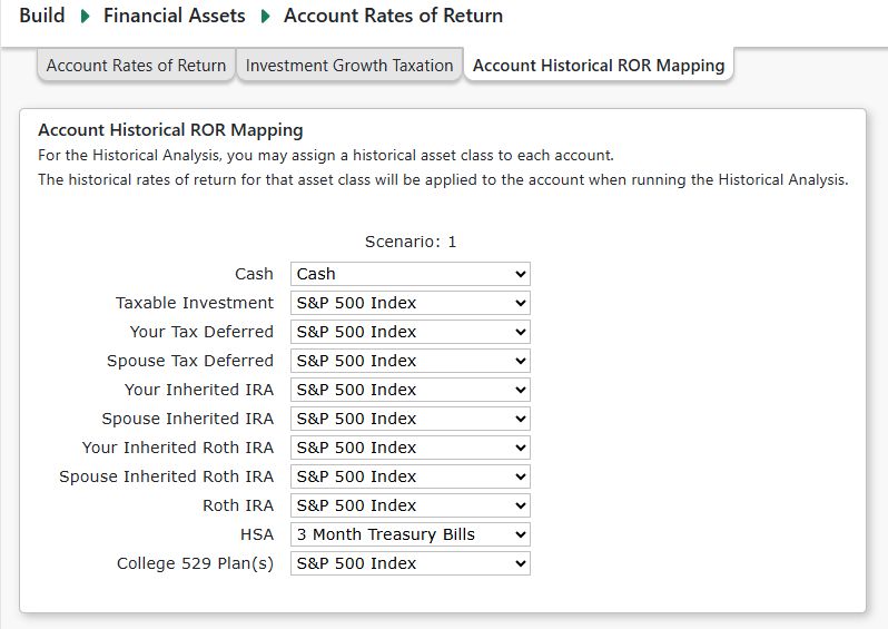
If your plan does have some negative cash flows, Pralana will list the years in which those occur and then present an output like that shown below.
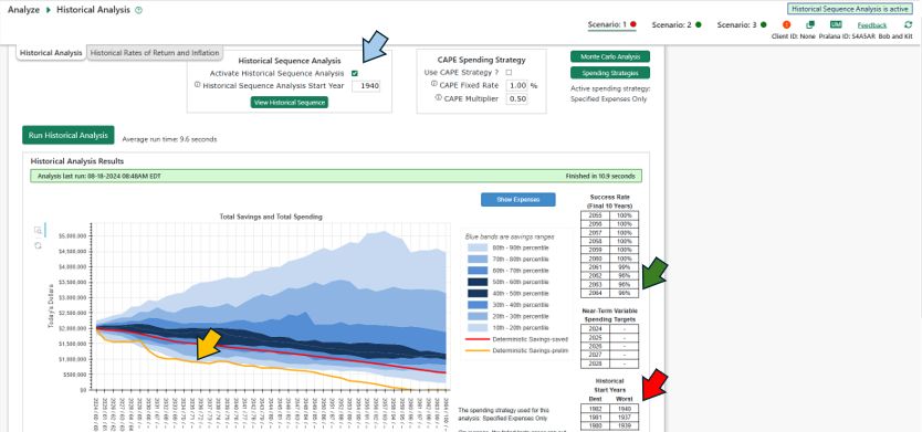
The objective of the optimization process is to maximize your final effective savings balance, and that is shown at the top of the section, along with the corresponding amount of improvement relative to your current settings (in terms of both dollars and percentage). Beneath that, it shows a number of different withdrawal priority options, ranked from best to worst and includes your current selections as specified on the Withdrawal Priorities tab of the Build > Financial Assets > Management page. In this example, the cursor was placed over the dot representing the best option and this has resulted in the pop-up box shown which identifies the final effective savings amount and other information.
If you want to replace your current withdrawal priority selections with the optimized settings, just click the Adopt Optimized Withdrawal Priority button. Clicking the button will render the display obsolete, so the optimization results display will disappear.
Another possible outcome of the optimization process is the one shown below, in which your plan runs out of money prior to the end of the modeling period regardless of the withdrawal priority. In this case, no optimization results are shown.
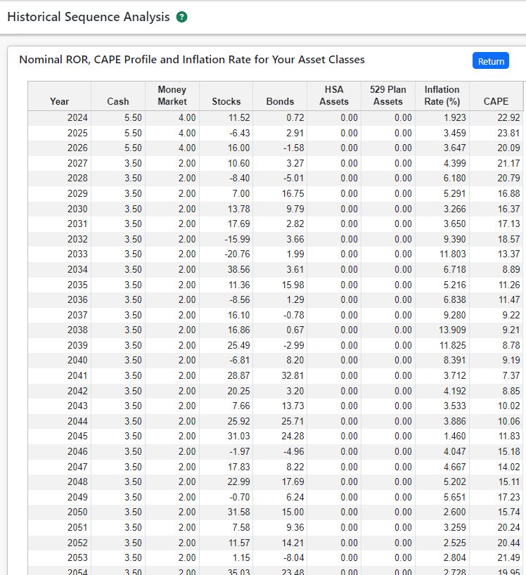
Optimization Results Table
One important thing to note is that there are up to 625 different withdrawal priority options and that many of these options yield the same final effective savings amount. The Optimization Results Table on this tab presents the complete set of results in tabular form. If you want to change your current setting to any particular one of these results, just click the Adopt button on the right side of the corresponding row in the table.
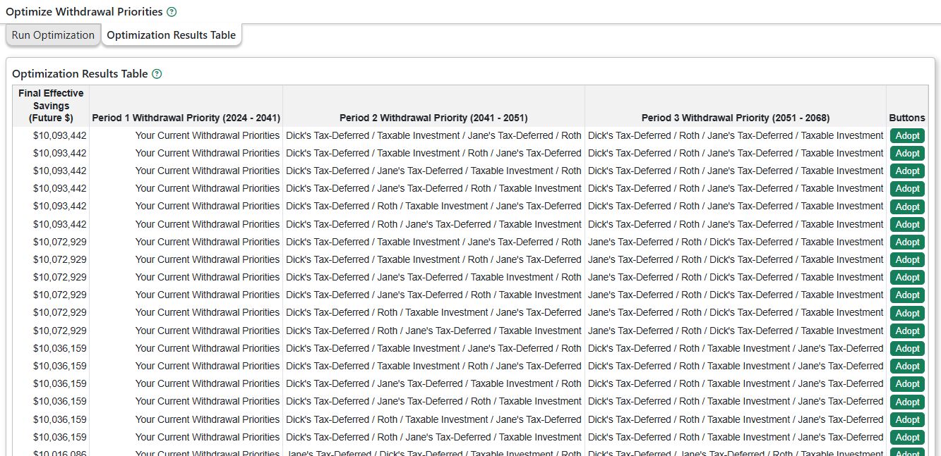
Earliest Safe Retirement Analysis
Pralana contains an advanced optimization algorithm that can help you select a retirement date. To do this properly, we need to be able to associate the end of pre-retirement income and expense streams and the beginning of post-retirement income and expense streams with that optimum retirement date. Rather than specifying a particular age, year or date to start or stop an income or expense stream (on the Income and Expense input pages), just enter the wild card character “R” (for Retirement). For pension, just enter “R” as your start date. The optimization algorithm will do the analysis to identify the date that keeps you from outliving your money in 90% of its test cases using the Monte Carlo analysis method.
Now let’s look at an example. To begin, you must ensure that your employment income stream(s) is associated with a designated retirement date, and this is done as follows. First, go to the Retirement & Life Expectancy tab of the Build > Get Started > Scenario Assumptions page, as shown below,
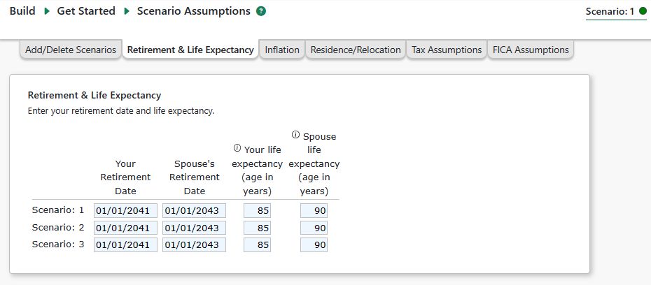
and enter your retirement date and your spouse’s retirement date. These are the dates on which you plan to cease full-time employment. Then, go to the Build > Income > Employment page and enter an “R” for the stop date on your employment income stream, as shown below. Although not shown here, you may also want to enter an “R” for the start date of another employment income stream or a pension stream, meaning that this is the date those streams are expected to begin.
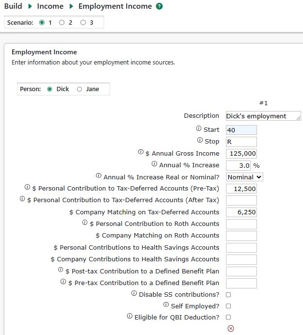
Note that the “Date at which full-time employment will cease” is currently set at 1/1/2041 and that Joe’s Employment Income Stream #1 begins at age 40 and extends to the designated retirement date (as indicated by the “R” in the Stop field. With the employment income streams set up we can proceed to the Analyze > Earliest Safe Retirement Analysis page. Just click the Run Earliest Safe Retirement Analysis button and Pralana will run repeated Monte Carlo analyses until it finds the retirement date that results in about 90% of the test cases ending with a positive savings balance. When it completes, you will see something like this:
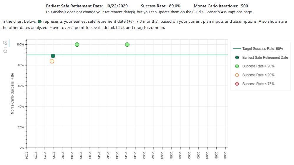
This graph shows the optimum solution of three slightly suboptimum solutions. At this point, the Earliest Safe Retirement Date of 10/22/2029 is just an “FYI”. If you want to incorporate this into your plan you will need to go back to the Retirement & Life Expectancy tab of the Build > Get Started > Scenario Assumptions page and manually insert this. If you were to do this and then go to the Analyze > Monte Carlo Analysis page and update the Monte Carlo analysis of your plan you then get a diagram that looks something like this:
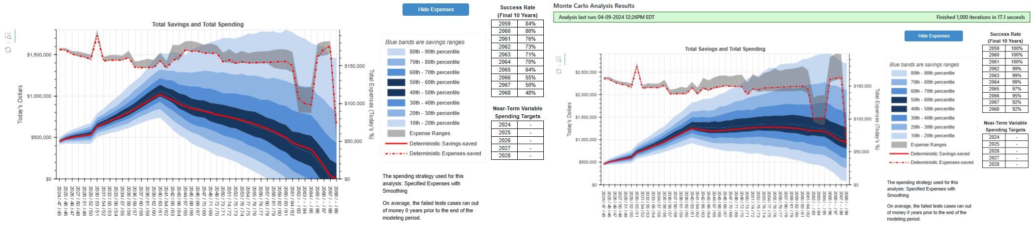
This analysis incorporates the early retirement date of 9/30/2023 and ends with a 92% success rate, about as expected. Every update of the Monte Carlo analysis will not end with a success rate of exactly 90% because of sequence of return variations from one run to the next but they should all be close.
Sensitivity Analysis
This analysis allows you to adjust selected scenario inputs and quickly see the impact on your scenario projections. Changes to sensitivity inputs only affect the ‘What If” projections shown on this page. They have no effect on you plan beyond this page. This page has 3 sections:
‘What if’ vs ‘Current’ Inputs
This section allows you to adjust various plan and scenario inputs by either entering a value or using the up and down arrows to adjust the ‘what if’ value by pre-determined increments.
Life Expectancy: Use this field to adjust life expectancy.
Retirement Start Date: Use this test changes to your retirement start date. The arrows will adjust the date in one year increments. Changing the retirement date affects any income or other inputs for which you enter ‘R’ as the start or end date. Also, it may affect the healthcare expense periods.
Social Security Start Age: Enter adjustments to Social Security enrollment age(s). Start ages must be between age 62 and 70.
General Inflation Rate: Enter an amount to be added to your general inflation rate for all inflation time periods. The up and down arrows will change the adjustment by 0.2% per click. Example: If your general inflation rate is 3.5% for 2025 and you enter an adjust of negative 1.0%, sensitivity projections will use a 2.5% general inflation rate (3.5% - 1.0% = 2.5%). The change will also alter healthcare, long-term care, college and other inflation rates which are based on apply to other inflation rates which are based on the general inflation rate. When you are using Simple Portfolio Modeling or Advanced Portfolio modeling with ‘real’ rates of return (RORs):
Adjustments to inflation rates will affect account/asset rates of return (RORs) because the adjusted inflation rate, along with your real RORs, are used to calculate the nominal RORs.
If you also enter a rate of return sensitivity adjustment (other than 100%), both adjusters will apply.
Rates of Return: This adjustment will change the nominal rates of returns used to calculate annual account growth. The arrows will change the adjustment in 2% increments.
Example 1: Using Advanced Portfolio Modeling (with nominal RORs), an account holds an asset ‘Stocks’ with a nominal ROR of 5.0% and you enter an adjustment of 90%. ‘Stocks’ nominal ROR will be 5.0% * 90% = 4.5%.
Example 2: Using Simple Portfolio Modeling (which uses real RORs), an account’s real ROR is 6.0% and you enter a adjustment of 120%. Assuming the inflation rate is 3.0%, the nominal ROR will be (3.0% + 6.0% + 3.0% * 6.0%) * 120% = 11.016%.
Note: when using real RORs, if you also enter a sensitivity adjuster for the general inflation rate, both adjusters will apply.
Consumption Smoothing Amount: This adjustment is only visible when using the Consumption Smoothing Spending Strategy. You may enter either a positive or negative amount. Negative amounts have the effect of applying a reduction to total expenses in each plan year. The arrows will adjust the Consumption Smoothing amount in $1,000 increments.
The background color of the input fields is light yellow if the value will change the scenario projections or light green, if not.
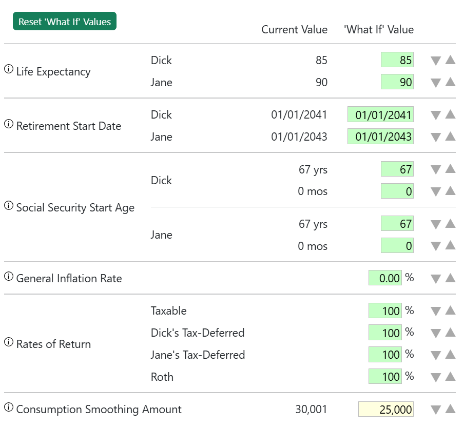
‘What if’ vs ‘Current’ Chart
The chart will show the impact of the sensitivity adjustments on your scenario projection for one of several metrics you may select in the Chart Metric dropdown list. The ‘Current’ line shows the projection using your current scenario inputs, without any adjustments. The ‘What If’ line shows the scenario projection with the adjustments applied. Notes:
If you have not made any adjustments, or only small adjustments, the lines will be the same or nearly the same and will overlap each other.
If you adjust your life expectancy, one line will be longer than the other. The X-axis labels will reflect the ages associated with the longer line.
Hover over the chart to see a popup showing the metric’s Current, What If and Different (in $ and %).
You may click and drag on the chart to zoom in. Click the reset button on the left to reset the zoom.
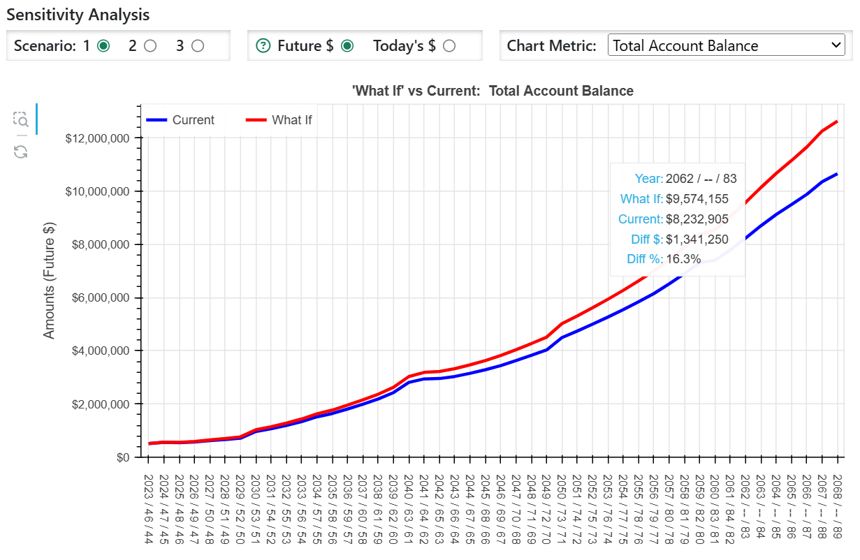
‘What if’ vs ‘Current’ Tabular Projection
This table will show selected What If and Current values of selected metrics. In the Table Metric dropdown, you may choose to show the same metric as in the chart, no metrics, or all the available metrics in the Chart Metric dropdown.
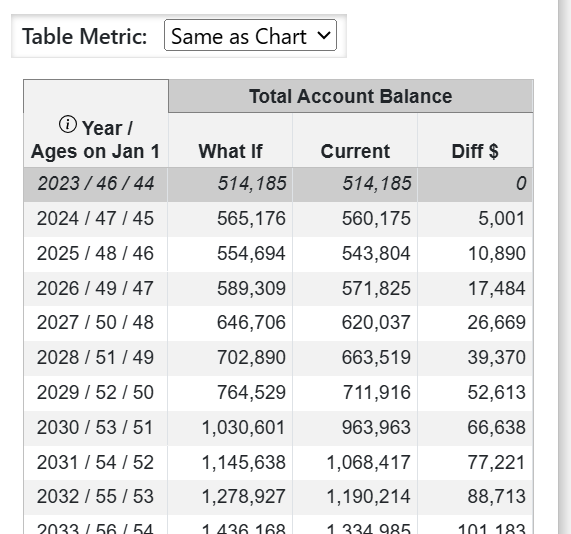
Reports
In addition to robust set of tabular and graphical projections discussed previously, Pralana also generates print-formatted PDF reports and renditions of IRS tax forms and other tax-related information.
Print-Formatted PDF Reports
Pralana enables you to create reports in PDF format for a selected scenario. One report will contain a summary of your inputs and the other will contain all the output tables and graphs generated from your inputs. These reports can be customized with the titles, subtitles, and page headers and footers of your choice, and can be formatted with either portrait or landscape orientation.
To create a PDF report, start by going to the Review > Reports > Reports Setup page which looks like this:
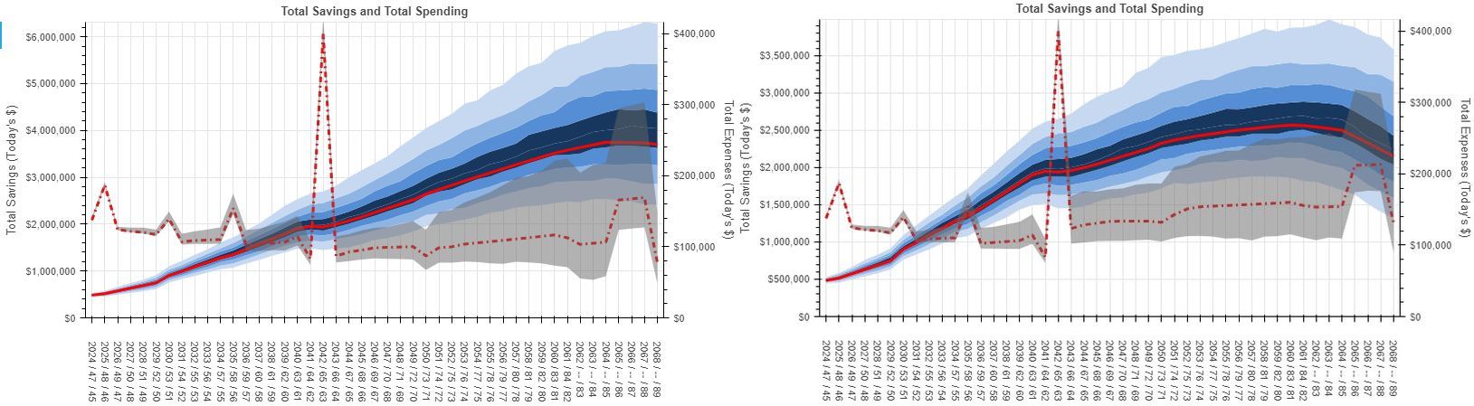
As you can see, there are several data entry fields on this page which allow you to specify the main title of the report along with two subtitles and multi-part page headers and footers. The information you enter on this page will apply to all scenarios.
To generate an input report, go to the Review > Reports > Plan Inputs Report page. Each report will be scenario-specific, and you can select the desired scenario via the control on the upper left of the Reports page. There are also controls on the page that enable you to specify paper size, portrait vs landscape orientation, and whether to hide unused input tables and fields. When you have the controls set as you desire, just click the Create Plan Inputs Report button and Pralana will generate your report. Here is a screenshot of that page prior to the report being run:
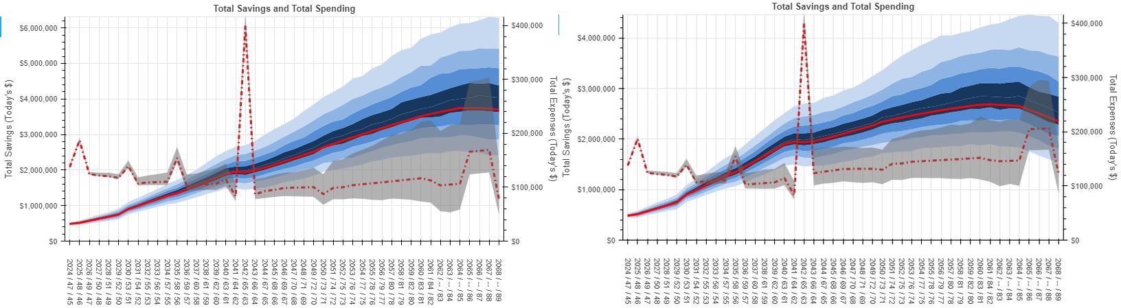
Here is a screenshot of the top portion of the page after the report has been generated:
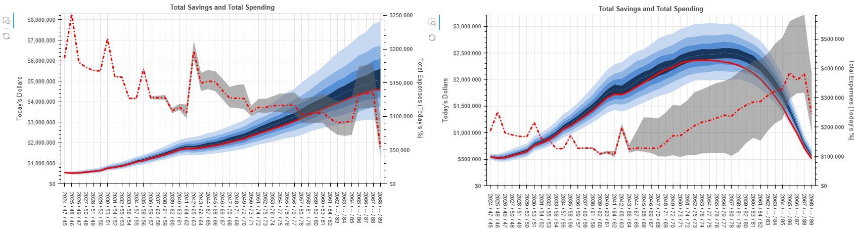
A preview of the entire report is shown on the same page where the report was initiated, and there are controls on the upper right of the window showing the report preview that enable you to save or print the report. If you click the “save” icon, you will get a page that looks like the one shown below where you need to specify that the report is to be printed to PDF and then specify your filename.
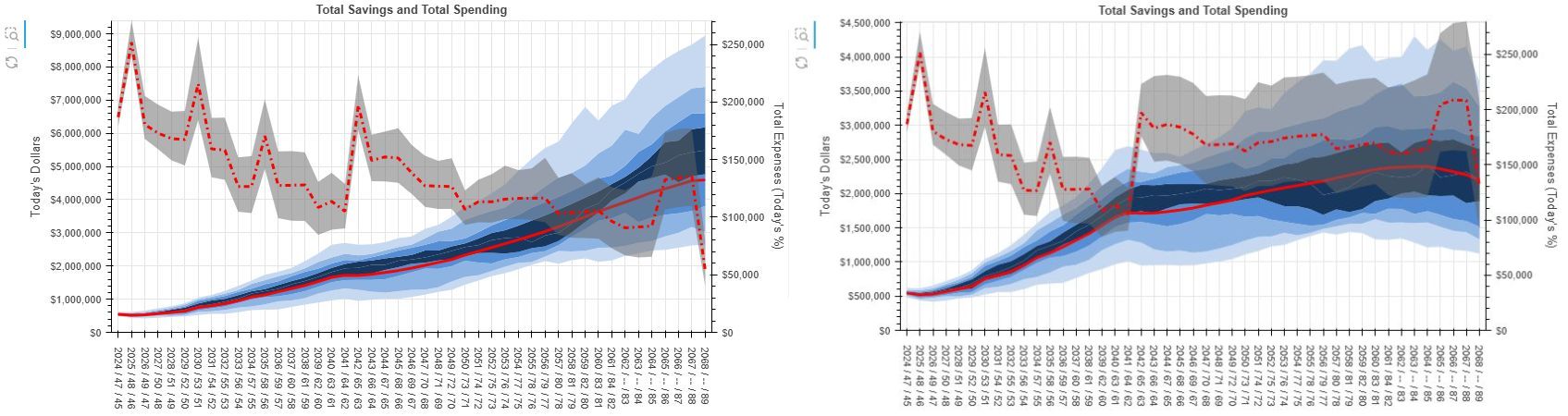
If you click the “print” icon, you will get a page that looks like the one shown below where you need to specify that the report is to be printed with margins set to “None” or “0”.
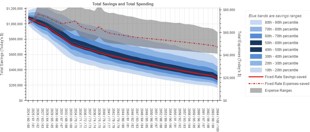
Alternatively, by clicking the “Open report in new browser tab” button, the report will appear in a separate tab in your browser, and you can examine it there while going on to a different page in Pralana. If you wish to print the report from the new browser tab, just use your browser’s print controls to do so. Here is an example of how to initiate that from MS Edge:
You start by clicking the 3 dots in the upper right corner of the browser window (this may be different on your browser):
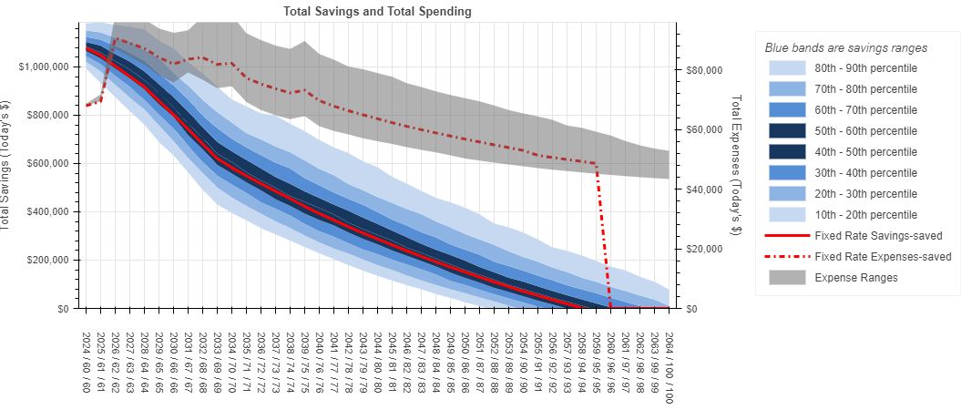
And this will cause a pop-up display like the one shown below, where you just click the Print option:
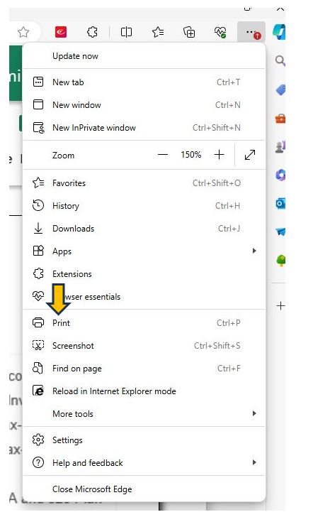
That will then bring up the pages where you can specify the destination for printing the report (i.e., either to a PDF file or to a printer) and the margin settings (always set to “none” or “0”).
Alternatively, there are other controls on the upper right of the window showing the report that enable you to save or print the report directly from the Review > Reports > Plan Inputs Report page. Regardless of the page from which you initiate the printing, please note that you will need to set the margins to “None” or “0” prior to printing.
To generate an output report, go to the Review > Reports > Plan Outputs Report page. Each report will be scenario-specific, and you can select the desired scenario and the preferred dollar units via the control on the upper left of the Reports page. There are also controls on the page that enable you to specify paper size and portrait vs landscape orientation and the remainder of the process is identical to that of printing plan input reports.
Tax Forms & Brackets
Pralana uses the information shown on these pages to calculate Federal, state and local income taxes.
As noted, these pages show how Pralana approximates future federal, state and local taxes. Pralana does not handle all provisions of the federal or state tax codes. We welcome suggestions for improving these approximations, within reason, as feature requests via Feedback using the ‘State Taxes’ category.
The Tax Forms page shows Pralana’s replica of various IRS tax forms. Select the a tax year from the drop-down and Pralana will show the forms available for that year.
The Tax Brackets page shows the Federal and State tax brackets as well as the LTCG brackets and the IRMAA brackets for the selected tax year.
The State Tax Parameters page shows Pralana’s rules and inputs for calculating state taxes for the selected state. See the Notes field for any custom coding to handle non-standard state provisions.
The State Tax Parameters (All States) page contains a table summarizing Pralana’s rules and inputs for calculating state tax for all states.
Advisor Capabilities
Pralana offers advisor subscriptions with 25, 50 or 100 client plans active simultaneously. Advisor subscriptions offer some features to help manage and client plans and to work collaboratively with clients on their plans.
Advisor Profile
This is the page where you can enter your name, contact information, and professional affiliations, and where you will see your Pralana advisor code. Here is a screenshot:
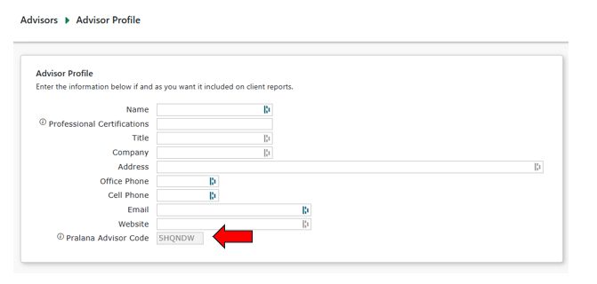
If you are working with a client who has his or her own subscription to Pralana and they wish to share their plan with you, you can give them your Pralana Advisor Code shown on this form. If they grant you permission to see their plan, it will appear in your list of client plans. You will be able to review and edit the plan as if it were your own, including changing inputs, copying scenarios, deleting the plan, etc. Shared plans will not count against the maximum number of client plans you are able to have in the tool.
Client Plans
To manage the plans for your clients, go to the Advisor > Client Plans
page. This will display a complete list of your plans and it enables you
to add, delete and select plans to be worked on. To add a client plan,
on the “new” row simply enter Client Name 1, Client Name 2 (if
applicable), and Plan Start Year. This action will cause a blank plan to
be created in Pralana for that client and the Pralana Plan Code will be
created automatically. To work on that plan, just click the Select
button and it will take you to the Build > Get Started > My Family page,
and you can navigate from there as desired. If you previously used
Pralana Gold and have export files for your clients, you will need to
create a plan for each of these clients in Pralana as just described,
and then import the data from Pralana Gold via the Build > Get Started >
Import PRC Excel Export File page. Once the plans have been created and,
if appropriate, populated via Pralana Gold imports, you can use Pralana
on the selected plan just as an individual user would use it for an
individual plan. To delete a plan, just click the icon
adjacent to the plan to be deleted and please note that this action is
irreversible.
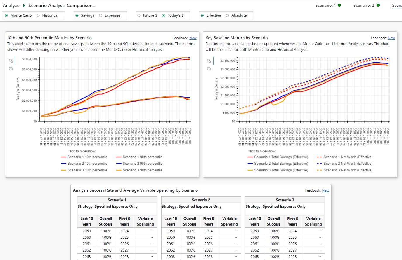
Data Security
We, at Pralana Consulting (“Pralana”), put a high priority on the privacy and security of your data. The information below describes, at a high level, the websites we operate and our data security practices. We will periodically update this document to provide more details and to reflect infrastructure changes.
Pralana operates two separate websites, hosted by different third-party vendors. These are:
Subscription Site: Our customer registration and subscription enrollment website is: www.pralanaretirementcalculator.com (‘Subscription Site’). You use this site to create your Pralana username, purchase paid subscriptions, download the Gold Excel-based Pralana Retirement Calculator, access the user forum and for other related activities. This site collects your name, email address, and payment information and maintains related information about your subscriptions.
Pralana Online: The web version of the Pralana Retirement Calculator is: www.pralana.online (‘Pralana’). On this site, you may enter information to create your Pralana financial plan, including first name(s), date(s) of birth and information about your assets, income and expenses. Pralana uses this information to make various financial projections and perform various analyses as described in the user manual.
Access to Pralana
You access Pralana by clicking a link on the Subscription Site, which acts as the Identity Provider (IdP). This link initiates a secure single sign-on (SSO) transaction to log you into Pralana. The only user information included in the SSO transaction is your Subscription Site username and the names of your active Pralana subscription plans. Authentication is performed using the username and x.509 security certificate information in the SSO transaction. Your full name, email address, physical address and payment information are not passed to Pralana.
Best Practices for Securing Your Data on Pralana
Safeguard your Subscription Site username and password and do not share them. Use a strong password.
First names are used to personalize the data entry pages and fields and column/row labels in reports, etc. You may enter “Me”, “Spouse”, “Child1” or other aliases. Do not enter full or last names.
Birth dates and years (for children) are used to calculate the start and stop dates of various income and expense cash flows. They are also used to estimate social security benefits, IRA required minimum distributions, eligibility age for qualified charitable distributions and similar age-based calculations. You may choose to enter a date other than your actual birth date. This may introduce some small inaccuracies, but if the date is close to your actual birth date, those inaccuracies will likely be immaterial.
Use generic financial account labels like “Checking”, “Savings”, “Bob’s IRA” etc. Do not enter your actual account numbers or other account access information.
For your homes and rental properties, use generic labels like “Current home”, “Shore house”, “Rental home 1”, etc. We suggest you do not enter identifiable property addresses.
Avoid entering personally identifiable information about your sources of income and expenses.
Pralana Website Hosting and Data Security
Pralana uses servers provisioned and managed by Render.com. User data is stored in a PostgreSQL database. The data is encrypted at rest using AES-256 data encryption in the database server and in the automated backups. Data is encrypted in transit using HTTPS secured by TLS certificates provided by Render.com. Backups are retained by Render.com for 7 days after they are created. More information about data security and trust at Render.com may be found at render.com/trust.
Pralana Consulting LLC Employees May Access Your Data
If you submit a question, suggestion or bug report we may access your plan or create a backup of your plan to investigate.
Appendix 1 – How Do I …?
This section poses and then answers some questions that we expect a typical user might ask.
How do I update my plan at the start of a new year?
At the start of each new year, you may change your plan’s start year at Build > My Family > About Me/Us or at Quick Start > Basic Plan Information. Here are some things to review and update, as needed:
Optional: Create a backup of your plan and/or create and download the plan inputs and results report PDFs.
On either the Quick Start or My Family page update the plan’s start year.
Update Account Initial Balances for all accounts, including unrealized LTCG and capital loss carryover on Taxable Investment accounts, and after-tax contributions on Tax-Deferred accounts.
Review all income and expense items for significant changes. A good way to do this is to create a Plan Inputs Report which has them all in one PDF which you can print. On the other hand, it may be useful to also look through each page that applies to you as new features may have been added (such as the ability to add inflation-adjustments to Phased Expense categories). In particular:
Review/update your Social Security benefit amounts to reflect the actual (if already started) or amount from the SS website.
Review property/rental property/investment/personal loan inputs. A ‘new’ loan can become an ‘existing’ loan and the inputs are different.
Review/update the Second Lowest Cost Silver Plan premium if you may be eligible for ACA tax credits.
Review your inflation assumptions on the Scenario Assumptions page, including the general inflation rate and adjusters for healthcare, long-term care, college expenses and Medicare premiums and IRMAA brackets. Also, review any Tax Assumptions you have made.
Review your portfolio allocation (for Advanced Portfolio modeling) and rate of return assumptions for the portfolio modeling method you are using.
Changes Pralana will make for you:
When you update your plan year, for example from 2025 to 2026, Pralana will automatically update the first time period (from 2025 to 2026) for inflation rates and adjustments, residence/relocation, phased expenses, portfolio time periods (used for Advanced Portfolio Modeling asset allocations and rates of return) and other time-period specific inputs. If you already have a time period defined for the new year (in this example 2026), those inputs will be retained and the 2025 settings will be deleted.
Model my income and FICA taxes?
Pralana does detailed calculations of your federal and state income taxes and your FICA taxes automatically, so it is virtually transparent to you. You do not need to specify any tax rates other than for any applicable local taxes. FICA tax calculations are a function of your employment and/or self-employment income, and Federal income tax calculations are a function of current tax tables, your AGI, marital status, itemized deductions and exemptions or your standard deduction, and your long-term capital gains. State income tax calculations are a function of current state tax tables, your Federal AGI, marital status, and state deductions and exemptions. If you would like to see the details for a particular year, you can visit the Review > Reports > Tax Forms page to see renderings of the relevant IRS forms, but please note that Pralana is not TurboTax; these are approximations.
Alternative Minimum Taxes and Net Investment Income Taxes are also calculated automatically.
Model contributions to my 401k? Roth account?
You can model contributions to your tax-deferred account (401k or IRA) and your spouse’s tax-deferred account (401k or IRA) via the Employment Income tab on the Build > Income page. The Employment Income tab is associated with a particular employment income stream and you can specify that contributions be made to your tax-deferred account and your Roth account from this income stream. Similarly, you can specify that your employer makes matching contributions to your accounts. There are specific input field for each of these for each income stream which you specify in terms of today’s dollars and these contributions will be increased annually at the same rate as the associated income stream.
These contributions go directly into the tax-deferred or Roth accounts and result in a corresponding reduction to this employment income stream. You can specify these contributions for an employment income stream that has no value if you want to model these contributions using some other form of income and, in this case, the contribution will be treated as an expense in the corresponding year.
Specify the amount I plan to save each month?
Annual contributions to your retirement accounts (tax-deferred and Roth accounts) are modeled based on your inputs on the Build > Income > Employment page, where you simply specify the annual dollar amount in today’s dollars. This can include your contributions as well as any company-matching contributions you may receive, and these annual amounts will be adjusted at the same rate as the corresponding employment income stream.
You cannot specify your annual contributions to either your cash account or your taxable investment account. Instead, the tool calculates those contributions so that every single dollar is fully accounted for in each year of the modeling period regardless of your cash flow. As we all know, your income and your expenses are not necessarily constant and, consequently, your cash flow varies from year to year. When it is positive, that excess money is modeled as a deposit to your cash account. When it is negative, the deficit is modeled as a withdrawal from your cash account. But the cash account has ceiling (i.e., upper) and floor (i.e., lower) limits, set by you, that govern the flow of money between the cash account and your other accounts. If deposits would tend to cause the cash account balance to exceed the ceiling level, the excess amount will be deposited in your taxable investment account. If withdrawals would tend to cause the cash account balance to go beneath the floor level, these withdrawals will be taken from other accounts in accordance with the withdrawal priorities you have specified on the Build > Financial Assets > Management page. Please refer to the section on Modeling Your Accounts for further information.
Model a pension?
Pensions are modeled via inputs provided on the Build > Income > Pensions page. You can model pensions as a lump sum or as an annuity simply based on the start/stop times. If those times are the same, the pension will be modeled as a lump sum; otherwise, the pension will be modeled as an annuity. Other input parameters (some of which only apply to annuities) are the pension amount and any COLA percentage, the percentage that will be rolled over to a traditional IRA or a Roth IRA and the percentage that is to be treated as non-taxable. You can also model survivor characteristics, such as the percentage your spouse will receive after your death or a Certain & Continuous period.
You can use a “wild card” to specify the start of your pension while using the same “wild card” to specify the end of your full-time employment income stream. Then, you can do what-if exercises to investigate the long-range effect of moving your retirement date forward or backward. This can be done in one or two ways: 1) By clicking up/down arrows to vary your retirement start age on the Analyze > Sensitivities page (sorry, this feature is coming soon but not available in the early releases of Pralana) or 2) by simply running an analysis on the Analyze > Earliest Safe Retirement Analysis page which will do a Monte Carlo analysis to determine the earliest retirement date that still allows you to not die broke with a 90% chance of success.
Model college educations for my kids?
You can model college educations for your kids via your inputs on the Build > Expenses > Children page. This page enables you to specify pre-college expenses for each of your children as well as their college educations. You can specify when you expect each child to start college, how many years he or she will be in college, total costs per year, and how this will be funded. The funding options modeled by the tool are pay-as-you-go, student loan, or 529 plan.
Model the downsizing of my home when I retire?
Pralana models your personal property, including homes, cars and recreational vehicles and all associated mortgages, purchase costs, taxes, insurance, maintenance and operating expenses, and sales costs. This is done on the Build > Expenses > Personal Property page. For each property, you simply specify when it was (or will be) purchased and sold, its cost basis and/or present value, details related to current or future mortgages, as well as all purchase, operating and sale expenses. Given that, the tool will model the purchasing and sale of all these properties along with their operating costs while you own them, as well as long-term capital gains as appropriate.
So, modeling the downsizing of your home is easy. Just enter the details of your current home and when you plan to sell it, and the details of your future home and when you plan to buy it and whether you plan to pay cash or get a new mortgage. The proceeds from the sale of your current home will be treated as income in the year it is sold, and the expenses associated with the purchase of your new home will be expenses in the year it is purchased. In effect, the tool will use the proceeds from the sale to purchase the new home and any money left over will be deposited in your Cash account. If that deposit pushes the Cash account balance over a specified ceiling, the residual will be deposited in your regular (taxable) investment account. The details of all these transactions can be found on the Review > Tabular Projections pages.
Model a reverse mortgage?
Pralana models your personal property, including homes, cars and recreational vehicles and all associated mortgages, purchase costs, taxes, insurance, maintenance and operating expenses, and sales costs. This is done on the Build > Expenses > Personal Property page. For each property, you simply specify when it was (or will be) purchased and sold, its cost basis and/or present value, details related to current or future mortgages, as well as all purchase, operating and sale expenses. Given that, the tool will model the purchasing and sale of all these properties along with their operating costs while you own them, as well as long-term capital gains as appropriate.
With that information in place, Pralana can model a reverse mortgage on a home. This is done via the Reverse Mortgage tab on the Build > Expenses > Personal Property page. Just select the property on which you want to model a reverse mortgage from a pull-down menu and enter the details of the reverse mortgage and the tool will put it in place. Visit the section in the manual on Modeling My Expenses for more information.
Model rental properties, including cash-out refinancing?
Pralana models your rental property, including all associated mortgages, purchase costs, taxes, insurance, maintenance and operating expenses, improvements, sales costs, depreciation, and rental income. It can also model cash-out refinancing. This is done on the Build > Expenses > Rental Property page. For each property, you simply specify when it was (or will be) purchased and sold, its cost basis and/or present value, details related to current or future mortgages, as well as all purchase, operating and sale expenses. Given that, the tool will model the purchasing and sale of all these properties, operating costs, improvement costs, depreciation, and rental income while you own them, as well as long-term capital gains as appropriate.
Model ACA health insurance?
Pralana models ACA health insurance using your inputs provided on the Build > Expenses > Healthcare page. The modeling period is broken down into up to five different time periods that correspond to life phases, such as 1) you and your spouse are both working full-time, 2) only you or your spouse are working full-time, 3) neither you nor your spouse are working full-time, 4) only one of you is eligible for Medicare and 5) both of you are eligible for Medicare. For the first four of these periods, you can specify whether you have ACA health insurance. Then, if you do, you can specify the premium you pay for your policy as well as the cost of the Second Lowest Cost Silver Plan in your area. Based on that, your healthcare MAGI, and your family size, Pralana will determine your Premium Tax Credit if you are eligible and will subtract that from your healthcare expenses, including your ACA premiums and any out-of-pocket costs you specify.
Model Medicare for my healthcare when I become eligible?
You and your spouse will become eligible for Medicare upon reaching age 65 and Pralana can compute your Medicare Part B premiums (including IRMAA) and your Medicare Part D surcharges and then include those with your other healthcare-related expenses. This is all controlled via your inputs on the Build > Expenses > Healthcare page, which contains two sections:
The section at the top is where you indicate whether you want the tool to automatically calculate your Medicare premiums and surcharges. If so, and if you or your spouse are already on Medicare at the start of the modeling period or will go on Medicare within the first two years, there are data entry fields through which you will need to specify your healthcare-related MAGI for the prior two years. This is necessary because Medicare premiums and surcharges are based on your MAGI from two years in the past, and the tool has no other way to know those numbers unless you simply tell it.
The section at the bottom deals with the variations in healthcare expenses as a person transitions from their working years, through their early-retirement years and on into their Medicare years. The tool defines up to five time periods to cover these transitions in which your costs can vary dramatically, and Periods 4 and 5 are the Medicare periods. In the fields on these rows of the table, you can specify any insurance premiums over-and-above the automatically-calculated premiums and your expected out-of-pocket costs.
Model a QCD?
A Qualified Charitable Distribution, or QCD, can be specified via the Build > Expenses > Charity page. On this page, you can define up to 10 charitable contributions, each of which may extend for multiple years. On any given row, the donation to a particular organization can be both a non-QCD and a QCD; if the donation begins prior to you turning age 70 ½, it will be treated as a non-QCD and when you reach age 70 ½, the donation will be treated as a QCD. A non-QCD is treated as an expense and is deductible as an itemized deduction. A QCD is not included in your expenses but, instead, results in a withdrawal from the specified tax -deferred account counts toward any RMDs.
Define my current assets?
You define your current assets via the Build > Financial Assets > Account Initial Balances page. There, you will find four tabs for defining your accounts in these categories: Taxable Accounts, Retirement Accounts, Health Savings Accounts and 529 Plans, and Inherited Accounts. Just click on any tab to enter the associated details.
On the Taxable Accounts tab, you can list your Cash accounts (such as your bank accounts) and their current balances, and your taxable investment accounts and their current balances, cost basis and any capital loss carryover.
On the Retirement Accounts tab, you can list your Roth Accounts and their current balances and traditional tax-deferred accounts for both you and your spouse and their current balances and any after-tax amounts that have been contributed.
On the HSA and 529 tab, you can list your HSA and 529 College Savings Plans and their current balances.
On the Inherited Accounts tab, you can identify one traditional inherited account for you and another for your spouse and one inherited Roth account for yourself and another for your spouse, along with the associated details.
Model my diversified portfolio and define the rate of return for each of my accounts?
Unlike most retirement calculators, Pralana does not ask you to specify the rate of return (ROR) for each of your accounts. To achieve its high-fidelity projections, Pralana utilizes asset classes, asset allocation and asset location processes and strategies to derive the ROR for each of your accounts. There are a variety of asset classes in which you could invest, each with different rates of return and levels of risk. Their returns can be correlated (move together), inversely correlated (tend to move in opposite directions) or uncorrelated. In taxable accounts, income from different asset classes may be taxed differently (as ordinary income, qualified dividends, or long-term capital gains). A diversified portfolio tends to have a mixture of asset classes with allocations that can vary over time in accordance with your risk tolerance. The challenge is to achieve your desired asset allocation while also optimizing long term wealth by holding asset classes in proper types of accounts. Pralana helps you achieve both goals.
To learn more about how this is done in Pralana, please refer to the section entitled Modeling Your Portfolio. It elaborates on the concepts of asset allocation and location and explains how to define your asset classes and specify the corresponding ROR, and how to select and specify one of two asset allocation modes that are then used to define the ROR for each of your accounts.
If you would prefer not to go to the level of detail associated with specifying asset classes and worrying about asset allocations, you can do that! Please see Simple Portfolio Modeling under Managing Your Portfolio for the details.
Model a Health Savings Account?
There are four elements to modeling a health savings account: entering the initial balance on the Build > Financial Assets > Account Initial Balances page, providing the investment details to enable the tool to derive the HSA’s rate of return on the Build > Financial Assets > Simple Portfolio Modeling page or Advanced Portfolio Modeling pages, entering future contributions via one of your employment streams on the Build > Income > Employment page, and then specifying pay-outs on the Build > Financial Assets > Scheduled Withdrawals page.
The tool does not make a direct connection between healthcare expenses and pay-outs; these are independent because you can allow your HSA to grow indefinitely and take withdrawals as you please. HSA withdrawals can be either qualified or unqualified and, either way, they will be deposited in your cash account. If the withdrawal is unqualified, it will be included in your AGI in the year the withdrawal occurs.
You can monitor the HSA contributions, withdrawals, and balance on the Review > Tabular Projections > Income and > Summary pages.
Model inherited IRAs and the associated RMDs?
Pralana can model one inherited traditional IRA for both you and your spouse and one inherited Roth IRA for both you and your spouse. These can be past or future inheritances and you have control over the way the RMDs are to be modeled. This is all controlled via your inputs on the Inherited IRAs tab of the Build > Financial Assets > Account Initial Balances page.
Model the taxes on the growth of my taxable account, particularly when it is invested in assets with different taxation properties?
The regular, taxable account can hold assets that are taxed in a variety of ways, including simple interest or unqualified dividends, qualified dividends, long-term capital gains (LTCG) that are taxed each year, tax-free, or as LTCG taxed only when withdrawn. To specify how the growth of the assets held in your regular taxable account are to be taxed, go to the Growth Taxation tab of the Build > Financial Assets > Portfolio page and specify that on an asset class basis. Pralana then apportions the growth of the taxable account based on these inputs and computes your taxes accordingly.
Model a loan to a family member?
If you have an outstanding personal loan, the pay-off of that loan can be modeled by Pralana. All you need to do is specify the current loan balance, APR and monthly payment, and the tool will model the amortization of that loan. All loan payments will be deposited in the cash account and the loan interest will be added to your AGI.
Tell Pralana how to deal with negative cash flows?
Your part in dealing with negative cash flows is to tell Pralana how to go about making withdrawals from your accounts to cover the deficit spending. You do this by specifying the withdrawal order via the table on the Withdrawal Priority subpage of the Build > Financial Assets > Management page. This table lists all your accounts in the order in which the tool will seek funds to cover a negative cash flow. The account at the top of the list is first priority and the other accounts are in descending priority order, with the lowest priority account at the bottom. To change the order, simply click on an account name and drag it to where you want it to be in the list and continue in this manner until the list is the way you want it.
When a negative cash flow occurs, the tool starts by trying to cover the deficit from the cash account; however, that withdrawal is only allowed to take the cash account balance down to the floor level and if more money is needed, then a withdrawal is made from the first account in the withdrawal priority list. When there is insufficient money in the first account, then the tool goes to the second account, and so on until the spending deficit is fully covered. Please refer to the section on Modeling Your Accounts for further information.
See what is causing my account balances to change each year?
The Review > Tabular Projections > Account Statements page provides a detailed breakdown of the contributions, growth and withdrawals that drive each of your account balances.
Know what goes into the AGI and itemized deductions that Pralana uses to calculate my income taxes?
There is a year-by-year detailed breakdown of both your Adjusted Gross Income and your Itemized Deductions on the Review > Tabular Projections > Expenses > Taxes page. There are separate tabs for these details.
Tell Pralana when to revert to pre-TCJA of 2017 tax laws?
The Tax Cuts and Jobs Act (TCJA) of 2017 is set to expire at the end of the year 2025, after which U.S. tax law will revert to the pre-TCJA of 2017 laws. Pralana implements both sets of tax laws and defaults to sunsetting of TCJA in 2025, but you can override it and specify any year in the future when the reversion to the pre-TCJA law will occur. This is done via the Tax Assumptions tab on the Build > Get Started > Scenario Assumptions page.
Model a relocation to a new state?
Pralana calculates state income taxes, so it needs to know your state of residence. It can model changes to your state of residence, as well. To do this, go to the Build > Get Started > Scenario Assumptions page and click on the Residence/Relocation tab. On this tab you can define your current state of residence as well as multiple residence changes in the future.
Additionally, this tab allows you to specify two other state-related items:
local tax rates, if applicable; these are combined with your state income taxes in all the tool’s projections
alternate state income tax rates if you find the tool’s state tax calculations are inaccurate; Pralana’s state tax calculations do not implement all the details of state taxes for 50 states plus the District of Columbia and the calculations for your particular state may be inaccurate as a result.
Model LTCG on the appreciation of my taxable account?
The regular, taxable account can hold assets that are taxed in a variety of ways, including simple interest or unqualified dividends, qualified dividends, long-term capital gains (LTCG) that are taxed each year, tax-free or as LTCG taxed only when withdrawn. To specify how the growth of the assets held in your regular taxable account are to be taxed, you go to the Growth Taxation tab of the Build > Financial Assets > Portfolio page and specify that on an asset class basis. Pralana keeps track of the unrealized LTCG in your taxable account and calculates the amount of LTCG included in any withdrawals made from that account and then calculates the appropriate taxes in the year those withdrawals occur. Visit the section in the manual on Modeling My Portfolio for more information.
Model market volatility and sequence-of-returns risks?
A Monte Carlo or an historical analysis is a good tool to test the viability of a retirement plan against a range of market environments and investment outcomes, including market volatility, and Pralana can do both types of analysis. These analyses use all the Financial assets, income and expense inputs you provide via the tool’s Build pages, but they replace the average returns used for the tool’s deterministic projections with either randomized or historical market returns to simulate market volatility.
Pralana’s Monte Carlo analysis generates 1000 independent projections using randomized annual rates of return for each of your accounts to simulate market volatility and aggregates these into a graph that illustrates the range of likely outcomes. The Monte Carlo analysis is on the Analyze > Monte Carlo Analysis page, and you can visit the section of the manual on Monte Carlo analysis for more information.
Pralana’s historical analysis generates 86 independent deterministic projections using historical inflation and historical rates of return for each of your asset classes to simulate market volatility and aggregates these into a graph that illustrates the range of likely outcomes. Additionally, the best and worst three historical sequences are identified and you can then use Pralana’s Historical Sequence Analysis capability to see the year-by-year details of the best and worst historical sequences in tabular form. The Historical analysis is on the Analyze > Historical Analysis page, and you can visit the section of the manual on Historical analysis for more information.
Both Monte Carlo and historical analyses are modeling sequence of return risks, but the Historical Sequence Analysis enables you to investigate the effect of a specific sequence of returns. See the next paragraph for more information.
Test my plan against a specific sequence of historical market returns, such as the one beginning in 1929?
Pralana’s historical analysis generates 86 independent deterministic projections using historical inflation and historical rates of return for each of your asset classes to simulate market volatility and aggregates these into a graph that illustrates the range of likely outcomes. You can then use Pralana’s Historical Sequence Analysis capability to highlight any particular sequence based on its starting year (say, 1929) to see it overlaid with the aggregation of all sequences. Further, you can see the year-by-year details of any specific historical sequence in tabular form. Visit the section on Historical analysis for more information.
Model a significant drop in the value of my portfolio immediately after I retire?
It is always a big concern if you plan to make withdrawals from your portfolio to meet your essential expenses and then there is a significant drop in the value of your portfolio early in your retirement. There are two fundamental ways of modeling this in Pralana to see just how big a potential issue this is.
One way is to use the Historical Sequence Analysis and select an historical sequence with particularly poor returns in the early years, such as 1929 or 1973. You can do this on the Analyze > Historical Analysis page and then see the resulting projection overlaid as a yellow line on the Historical Analysis range of outcomes (the blue bands) and the deterministic projection (the red line) produced with average rates of return. With the Historical Sequence Analysis mode active, you can also see the detailed results on all the tabular projections pages.
Another way is to manually define and specify a sequence of returns for each of your asset classes via the Build > Financial Assets > Portfolio pages. These pages enable you to define different rates of return for all your asset classes for a specified number of different time periods, and you can do this on a per scenario basis. If you choose this option, the result will be reflected in the tool’s deterministic analysis outputs: all the tabular projections pages and the red line on the graphs on the Monte Carlo and Historical Analysis pages.
Model different spending strategies in my retirement years?
Pralana can model your spending exactly as you specify it on the Build > Expenses pages, but very importantly, it gives you the option of replacing your specified non-essential spending with variable spending in your retirement years. This capability uses several alternate spending strategy algorithms to dynamically vary your spending as a function of the performance of your portfolio. No doubt, you would not maintain your specified spending level while watching the value of your portfolio go to zero, so these algorithms give you some options to model what you would you likely do in real life depending upon how your portfolio performed.
A deterministic analysis of your plan with specific income, expenses, and portfolio performance is a great way to evaluate its fundamental viability. In the real world, though, if your portfolio was underperforming your expectations, you probably would not just continue spending at the same level as if everything was rosy while watching your net worth go to zero. Similarly, if it was outperforming your expectations, you might elect to live it up a bit. You would most likely adjust your spending over time as a function of your portfolio’s performance to avoid outliving your money, and Pralana enables you to model that behavior and gives you actionable near-term spending targets. If you want to do this, start by going to the Analyze > Spending Strategies page. There, you will find the controls for telling the tool that you wish to use one of eight (8) alternate spending strategies rather than the fixed spending specified on the Build > Expenses pages. Please refer to the section on Variable Spending Strategies for more information.
Determine when I can retire?
Pralana has various ways of exploring this question, and all are based on use of a “wild card retirement date” to define the end of your full-employment income stream and the start of your pension, if applicable. This effectively connects your income streams such that you can adjust the starts and stops by changing only one variable. Then, you can conduct studies based on variations in that “wild card retirement date” and you can optimize the “wild card retirement date” to a specific date that yields a 90% success rate of not dying broke based on Monte Carlo analyses.
Initially, you will specify your planned retirement date and your spouse’s planned retirement date on the Build > Get Started > Scenario Assumptions page. Next, you will need to associate the end and/or beginning of selected income streams with these retirement dates. You do this by entering the character “R” in the start or stop fields of any Employment, Pension, Annuities or Other Income streams on the Build > Income pages.
There are now two ways you can adjust the “wild card retirement date” to explore the “when can I retire” question.
The first is obvious: simply go back to the Build > Get Started > Scenario Assumptions page and manually modify the date, and then go to the Review > Tabular Projections > Balance Sheet page and examine the effect on the deterministic projection of your total savings over time. You can also go to the Analyze > Monte Carlo and > Historical Analysis pages and run analyses to check out the likely range of outcomes based on your retirement date(s).
You can also go to the Analyze > Earliest Safe Retirement Analysis page and simply click the “Run Earliest Safe Retirement Analysis” button and the tool will automatically determine the earliest value of the “wild card retirement date” that results in a success rate of 90% that you will not outlive your money. If you elect to use this information as a basis for selecting your retirement date(s), you will need to go back to the Build > Get Started > Scenario Assumptions page and make those changes.
Model various alternative retirement dates and explore the long-term viability of each alternative?
You can use a “wild card” to specify the start of your pension while using the same “wild card” to specify the end of your full-time employment income stream. Then, you can do what-if exercises to investigate the long-range effect of moving your retirement date forward or backward. This can be done in one or two ways: 1) By clicking up/down arrows to vary your retirement start age on the Analyze > Sensitivities page or 2) by simply running an analysis on the Analyze > Earliest Safe Retirement Analysis page which will do a Monte Carlo analysis to determine the earliest retirement date that still allows you to not die broke with a 90% chance of success.
Please see the paragraph entitled “Options for Defining the Start and Stop of Income Streams” under the Modeling Your Income section for more information.
Do consumption smoothing?
Consumption smoothing is an algorithm that helps you maximize your standard of living over the remainder of your life in such a way that you will not have to starve now to live in luxury during retirement, or vice versa. More specifically, this algorithm considers all the assumptions, income and expenses you have already entered into the tool and then calculates a “delta” expense value such that the whole of these parameters represents the maximum sustainable standard of living that can be supported over your entire lifetime.
You can read more about this concept and its real-life application in the book entitled “Spend ‘til the End” by Laurence Kotlikoff and Scott Burns.
An alternative and equally important use of Pralana’s consumption smoothing capability is to gain insight into the amount of margin that exists in your plan. If you wish to explore consumption smoothing, it is selectable via the pull-down menu on the Analyze > Spending Strategies page.
Model survivor scenarios?
Pralana contains a variety of features that enable you to model and evaluate survivor scenarios. The first thing you need to do is be aware of the way the tool models the death of a marriage partner, as shown below, and ensure that your Build page settings are correct:
Employment income streams are terminated upon the death of the owner
Pension income streams with survivor benefits or that are still within the Certain & Continuous period will be converted to a pension for the survivor, as appropriate
Social Security benefits are terminated upon the death of the owner, but those benefits may replace the survivor’s prior benefits if it results in a higher benefit
Annuities with survivor benefits will become annuities for the survivor upon the death of the owner, as appropriate
If the decedent has term life or cash value life insurance, it will be paid to the survivor as a deposit to the cash account
ACA premiums will change as a function of the smaller family size and Medicare premiums will be cut in half. Finally, there is a control on the Build > Expenses > Healthcare page that allows you to specify a healthcare expense reduction percentage that goes into effect upon the death of a partner (but does not affect ACA and Medicare premiums which are handled independently).
There is a control on the Build > Expenses > Phased page that allows you to specify a phased expense reduction percentage that goes into effect upon the death of a partner.
With all the above settings in place, there are multiple ways to evaluate survivor scenarios:
You can easily change the life expectancy for either marriage partner on the Retirement & Life Expectancy tab of the Build > Get Started > Scenario Assumptions page, and you can do this independently for each scenario. So, you can simply make the desired change and then go look at the deterministic projection and examine the details to check on cash flow and how the account balances behave. You can then run a Monte Carlo analysis to look at long range outcomes and ensure they are still in positive territory.
You can set different life expectancies on the three scenarios, then run Monte Carlo analyses on each of them and then go to the Analyze > Scenario Analysis Comparisons page to see graphical overlays to see how the different scenarios compare in the long term.
Use Pralana to evaluate alternatives and make key financial decisions?
It is extremely easy to evaluate and compare alternatives that will facilitate key financial decisions. This is based on the concept of a “scenario”, which is defined to be the complete set of assumptions and parameters used to govern the tool’s projections. The key to evaluating alternatives is that Pralana models three independent scenarios simultaneously and allows you to overlay the projections of all three scenarios on the same graph to see how they compare.
Some of your inputs apply to all scenarios, such as your marital status,
birthdate(s), children, and initial account balances. Nearly all other
parameters are scenario-specific and on most pages you will see a set of
radio buttons that enable you to select the scenario to which the inputs
on that page apply. In a few cases, the inputs for all the scenarios are
visible at the same time. With this capability, you can define the
details of each alternative you wish to model. Presumably, all your
scenarios will be similar but with one or more key differences. To
facilitate the creation of these different scenarios, you can start by
defining a base scenario (say, scenario #1), then invoking the tool’s
global copy function (i.e., by clicking the 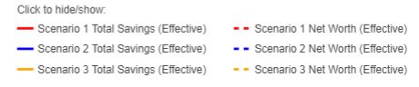 icon) to create
an identical scenario (say, scenario #2) and then again to create
another identical scenario (say, scenario #3). Then you can go to the
Build pages and make whatever changes you wish to make to scenarios 2
and 3 to create the other alternatives to want to explore.
icon) to create
an identical scenario (say, scenario #2) and then again to create
another identical scenario (say, scenario #3). Then you can go to the
Build pages and make whatever changes you wish to make to scenarios 2
and 3 to create the other alternatives to want to explore.
With the data input done, you can then go to the Analyze > Monte Carlo Analysis or > Historical Analysis and run those analyses on each of the three scenarios. Then you can go to the Analyze > Scenario Comparisons page to see the overlaid projections and use that information to help make your decisions. Additionally, you can go to the Review > Tabular Projections page and examine the details of each of your scenarios. You cannot see direct comparisons this way, but you can see the year-by-year details of a given scenario, selected via the radio buttons at the top of the page.
Model life insurance?
Pralana models term life insurance and cash value life insurance for both you and your spouse. This is all done via the Build > Expenses > Term Life Insurance and > Cash Value Life Insurance pages. Visit the section in the manual on modeling Life Insurance for more information.
Delete My Data?
If you decide you want to delete your data from Pralana, there is a mechanism to do it. Just go the More > Delete My Data page and click the “Delete my Plan data” button. This will delete your existing plan from the Pralana database and replace it with a sample plan for you and your spouse. Please be aware that there is no recovery from this process. Once your plan is deleted, there is no going back.
Get help in using Pralana Online if I need it, or if I would just like a knowledgeable third party to review my plan with me?
In addition to this user manual, you can get help via the Pralana Forum or by engaging one of the fee-only financial advisors listed on the Pralana website.
Appendix 2 – Future vs Today’s $
Borrowing from Wikipedia:
“Present value is the concept that states that an amount of money today is worth more than that same amount in the future. In other words, money received in the future is not worth as much as an equal amount received today.
Inflation is the rise in prices of goods and services over time. If you receive money today, you can buy goods at today’s prices. As inflation causes the price of goods to rise in the future, your purchasing power decreases. Consequently, money that you don’t spend today could be expected to lose value in the future by some implied annual rate (which could be the inflation rate or the rate of return if the money were invested).
Where FV = future value, r = rate of return, and n = number of periods.
Here is an example:
Let’s say you have the choice of being paid $2,000 today earning 3% annually or $2,200 one year from now. Which is the best option?
Using the present value formula, the calculation is $2,200 / (1 +. 03)1 = $2,135.92
PV = $2,135.92, or the minimum amount that you would need to be paid today to have $2,200 one year from now. In other words, if you were paid $2,000 today and it could earn a 3% interest rate, the amount would not be enough to give you $2,200 one year from now. Therefore, you would be better off to take the $2,200 one year from now.
A comparison of present value with future value (FV) best illustrates the principle of the time value of money and the need for charging or paying additional risk-based interest rates. Simply put, the money today is worth more than the same money tomorrow because of the passage of time. Future value can relate to the future cash inflows from investing today’s money, or the future payment required to repay money borrowed today.
Future value is the value of a current asset at a specified date in the future based on an assumed rate of growth. The FV equation assumes a constant rate of growth and a single upfront payment left untouched for the duration of the investment. The FV calculation allows investors to predict, with varying degrees of accuracy, the amount of profit that can be generated by different investments.
Present value is the current value of a future sum of money or stream of cash flows given a specified rate of return. Present value takes the future value and applies a discount rate or the interest rate that could be earned if invested. Future value tells you what an investment is worth in the future while the present value tells you how much you’d need in today’s dollars to earn a specific amount in the future.
The Bottom Line: Present value is a way of representing the current value of future cash flows, based on the principle that money in the present is worth more than money in the future. Present value is used to value the income from loans, mortgages, and other assets that may take many years to realize their full value. Investors use these calculations to compare the value of assets with very different time horizons.”
Appendix 3 – Modeling Market Volatility, Multiple Asset Classes, and Annual Rebalancing in Monte Carlo Simulations
This appendix explains how Pralana models market volatility in Monte Carlo simulations, why Monte Carlo “typical” outcomes (for example, the 50th percentile/median) can differ from deterministic projections, and why the difference can become more noticeable when a portfolio contains multiple volatile asset classes.
Geometric vs. Arithmetic Returns: Why the Distinction Matters
A deterministic projection applies a constant annual rate of return to account or asset balances. Whether entered directly as a nominal return or derived from a real return and inflation assumption, this rate represents the expected compound growth rate of the investment. Because balances grow multiplicatively from year to year, the entered return is interpreted as a geometric mean return (often informally called CAGR).
Monte Carlo simulations, in contrast, model returns as random year-by-year outcomes. In this context, there is an important difference between:
the geometric mean return (the compounded growth rate over time), and
the arithmetic mean return (the simple average of annual returns).
Under commonly used assumptions, the arithmetic mean exceeds the geometric mean by an amount related to variance:
Approximation: Arithmetic mean ≈ Geometric mean + (Standard Deviation²)/2
Pralana treats asset-class rates of return entered by the user as geometric (compound) return assumptions, which are used for deterministic projections. For Monte Carlo simulations, Pralana uses the corresponding standard deviations to estimate an arithmetic mean that is consistent with the specified geometric return assumption and then generates randomized annual returns from that distribution. This calibration ensures that, for a single asset class, the long-term expected compounded growth in Monte Carlo simulations is consistent with the user’s specified return assumption.
Volatility Drag: Why “Average Return” Isn’t the Whole Story
Volatility drag is the phenomenon that higher volatility tends to reduce compounded growth (geometric return), even when the simple average (arithmetic) return is unchanged. This is one reason deterministic projections (which use a single compounded rate) and Monte Carlo results (which include volatile year-by-year paths) can differ.
Pralana’s approach—using geometric assumptions for deterministic projections and using an arithmetic mean for Monte Carlo return generation—helps align the stochastic modeling with long-term compounding behavior.
Annual Rebalancing + Multiple Asset Classes Can Increase Compound Growth
Because Pralana rebalances asset classes each year, multi-asset portfolios can exhibit a well-known effect called:
diversification return,
rebalancing bonus, or
volatility pumping.
Intuitively, when two (or more) volatile assets do not move in perfect lockstep, annual rebalancing tends to:
trim assets that rose relative to the target, and
add to assets that fell relative to the target,
restoring the intended asset allocations.
When asset-class returns are not perfectly correlated, this disciplined “sell high / buy low” mechanism can increase long-term compound growth even if the asset classes have similar long-run return assumptions.
This effect is typically:
stronger when volatility is higher, and
stronger when correlations are lower (i.e., when assets move more independently).
What Users Should Expect (Key Observations)
Given that Pralana always rebalances annually, the following patterns are common:
1. Single asset class (or effectively one risky return stream):
There is little or no opportunity for rebalancing to add compound growth across asset classes. Monte Carlo medians often appear closer to deterministic projections (while still showing a wider spread with higher volatility).
Practical Guidance and Interpretation
A higher Monte Carlo median than deterministic does not necessarily indicate an error. It may reflect the mathematical impact of combining:
multiple volatile assets,
low correlation between those assets, and
Pralana’s annual rebalancing to target allocations.
If a user models multiple “stock-like” asset classes as uncorrelated and with high volatility, the model may show a large rebalancing bonus that would not occur if those assets were highly correlated in the real world.
Users should interpret Monte Carlo results in light of whether the assumed correlation between asset classes is realistic for their portfolio.
Summary
Pralana’s deterministic projections use user-entered asset-class return assumptions as geometric (compound) returns. Monte Carlo simulations generate year-by-year random returns using an arithmetic mean derived from those assumptions and each asset class’s volatility. Because Pralana rebalances asset classes annually, a portfolio with multiple volatile, uncorrelated asset classes can experience a diversification return that raises long-term compound growth. This can cause Monte Carlo median outcomes to exceed deterministic projections, especially in high-volatility scenarios.
Appendix 3 – Restore from Backup Reference
Backup files are encrypted and contain plan inputs as well as the plan owner’s username, your username, plan code, date/time of backup, Pralana Online site version, and each scenario’s final savings.
Restoring from backup may update your currently active plan, create a new plan or do nothing, as described in the table below.
Platinum (single plan) subscribers: You may restore backup files you created, if the plan code in the back up matches your current plan’s code1.
Subscr iption/ user type* |
Plan code in .pral ana_backup file matches user’s currently active plan? |
Plan count sta tus* |
Ad diti onal plan cr eate d? |
User’s cu rrently active plan is…* |
Plan code after res tore |
Notes |
|---|---|---|---|---|---|---|
Single Plan* (Plat inum) |
Yes |
n/a |
No |
R eplaced |
Same |
|
No |
n/a |
No |
Un changed |
n/a |
Restore blocked 1, 2 |
|
A dvisors (P latinum Pro) and Family Plan |
Yes |
n/a |
No |
R eplaced |
Same |
|
No |
Below ma ximum |
Yes |
Un changed |
New code |
New plan added |
|
No |
At ma ximum |
No |
Un changed |
n/a |
Restore blocked |
|
** Staff** |
Yes |
n/a |
No |
R eplaced |
Same |
|
No |
n/a |
Yes |
Un changed |
New code |
New plan added |
1 If you adopted another user’s plan and later need to restore a backup from before the adoption, the plan codes will not match and the restore will be blocked. In this case, email your pre-adoption backup file to mail@pralanaconsulting.com and our team will restore it for you after verifying your ownership.
2 Pralana will restore plans with mismatched plan codes for single-plan beta testers on the test website.
Restore Verification: After the restore, Pralana calculates the restored plan’s projections and final savings and shows a comparison of the savings at the time of backup versus the restored file. It is normal for the backup/restore savings to differ if the site has been updated since the backup was created. Site version updates may change tax information, add or change features, and affect projection calculations.
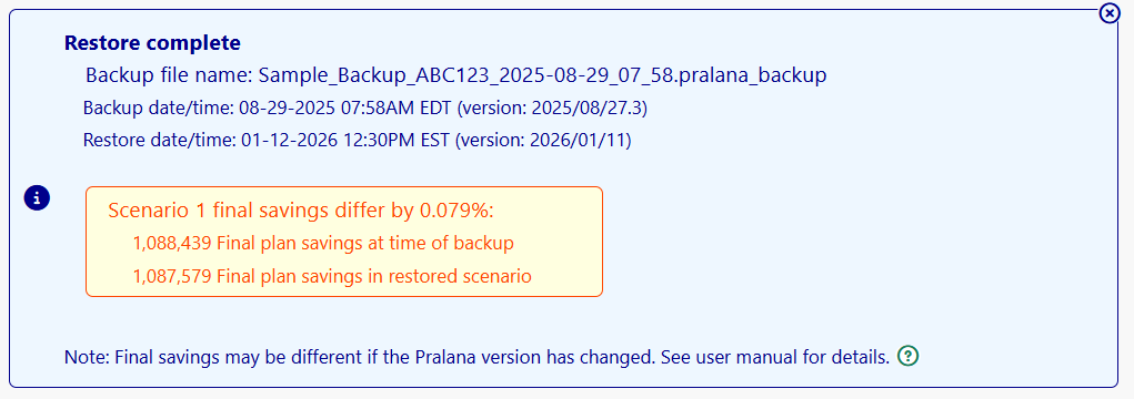
Verification Failures: As a safety precaution and to protect your current plan’s data, Pralana will abort the restore if the backup/restore savings do not match and the backup/restore site version are the same. This should never occur and indicates a problem. The original plan remains unchanged and the user is alerted.
Social Security Benefits
Pralana goes way beyond simply asking you to specify benefit amounts and start ages. Based on the information you provide, Pralana will calculate:
Your and, if applicable, your spouse’s, Social Security benefit adjusted for early-filing reductions and delayed filing credits based on your start date (if not already started)
Spousal supplement (if not already started)
Survivor benefit, if applicable.
Deferred and make-up benefits due to excess employment income
Enter the age (year and month) at which you and your spouse, if applicable, did or will start taking benefits.
If your benefits have not yet started and:
you have not yet reached your Full Retirement Age (FRA), enter the monthly benefit shown on the SSA website for your FRA.
you are already past your FRA, enter the monthly benefit shown on the SSA website for age 70.
If your benefits have already started, enter the actual monthly benefit amount you receive, including any spousal supplement.
Pralana follows the SSA’s rules for ‘attained age’ and that benefits are paid one month in arrears (e.g. the benefit you earn in January is not received until early February. Performing these calculations provides these benefits:
Easy what-if exercises: by simply changing your and your spouse’s start ages, you can quickly observe long term effects on your net worth without having to figure out and then enter the corresponding changes to benefit amounts.
Enables Pralana to compute the optimum ages for you and your spouse to begin taking SS benefits (for more information, see the Analyze > SS Optimization page).
Spousal Benefits
If an eligible person has not yet started benefits and their spouse starts benefits before their own start date, Pralana will calculate their spousal benefit.
Survivor Benefits
Survivor benefits may start as early as age 60. In a two-person plan, when the first spouse is deceased, Pralana assumes the survivor will start survivor benefits immediately if their own benefit has not already started. In a one-person plan where the person’s spouse died prior to plan start, Pralana provides the option for the person to indicate that they are receiving survivor benefits at the start of the plan.
When a person receiving survivor benefits reaches their own start age, Pralana will give the person the greater of the survivor benefit of their own benefit (adjusted for any early or delayed start of benefits).
Excess Employment Income
If a person has started benefits prior to their full retirement age and receives employment income over the limits established by the Social Security Administration, Pralana will defer some or all of the Social Security benefit until the person reaches full retirement age. Thereafter, the accumulated deferred benefit will be paid out over some years. If applicable, the Social Security benefit projections will show the amounts of deferred and makeup benefits.
Note: In the first year of retirement, Pralana assumes employment wages are evenly distributed across the year. It does not implement Social Security’s Special Earnings Limit Rule, which allows benefits to be paid in months when you are “retired” under a monthly earnings test even if total annual wages exceed the annual limit.
Field-by-Field Description of Social Security Income Inputs
Full Retirement Age: For your reference, your full retirement age (FRA) is calculated by Pralana based on your date of birth.
Check if not eligible for Social Security benefits: Check this box if you are not eligible for SS benefits because of participation in some other retirement program. This will prevent spousal benefits from being generated automatically by the tool.
Age at which you did or will start benefits: If this age is still in the future, it will be used to determine your future benefit; if this age has already passed and your benefits have already started, it will be used to determine potential spousal benefits.
Monthly Benefit Amount: Monthly benefit in today’s dollars. See below for more details about the amount to enter. Leave it blank if this person has no benefits of their own; Pralana will calculate spousal benefits based on the other spouse’s work record.
Benefit amount entered is: Select one of these options:
Actual benefit (already started): Enter the monthly amount received as of the plan start date (including any spousal benefit).
Benefit at FRA (not started): Enter the benefit shown on the Social Security Administration’s website for your full retirement age. This amount is only available if you have not yet reached your FRA.
Benefit at 70 (not started): If you are older than your FRA, enter the benefit shown on the Social Security Administration’s website assuming you start benefits at age 70.
Annual Survivor Benefit Amount: (for plans with Marital status = ‘Single’) This field allows a widow/widower to enter the Social Security survivor benefit they are collecting based on the earnings record of a spouse deceased prior the plan start.
Note: The GPO spousal reduction was repealed by legislation in early 2025.
Social Security Disability Modeling
Pralana does not specifically model Social Security Disability benefits. If you need to do this, we recommend using two Other Income streams: one to represent the taxable portion of the SSDI stream and another to represent the non-taxable portion of the SSDI stream. Determining how much of your SSDI is taxable and how much is non-taxable is a function of your MAGI and is an exercise you will need to perform outside of PRC. The maximum taxation on any SS income is 85%, so a worst-case way to go would be to set Other Income #1 (taxable) to 85% of your SSDI and Other Income #2 (non-taxable) to 15% of your SSDI.
One-Time Benefit Reduction
If you want to model a one-time Social Security benefit reduction at some point in the future, you can do that on the Social Security Income page. There is a section on the lower right portion of the page through which you can specify the year in which this is to occur and the percentage by which your benefits are to be reduced. Just leave these fields blank if you do not want to model a benefits reduction. As an example as to how this works mathematically, if you specify a 10% reduction, Pralana will calculate your benefits and then multiply that by (100%-10%), or 0.9.
Cost of Living Adjustments
By default, Social Security benefits are modeled to increase at the general inflation rate. If you want to model a different COLA rate, you can do that on the Social Security Income page. There is a section on the lower left portion of the page through which you can specify the year your preferred rate is to begin and the addition or reduction percentage relative to your general inflation rate. For example, if the general inflation rate is 3% and you believe SS benefits will increase at 2%, enter a “-1%” in this field. Just leave these fields blank if you want Social Security benefits to be adjusted at the general inflation rate.
Benefit Projections
Based on the inputs you have provided, Pralana generates an output table to show you the resulting Social Security benefits on an annual basis, like the example shown below.
Note that spousal benefits are shown when appropriate and that the values in the Social Security Income column are underlined. This means that the Metric MRI is available and that if you click on that value you will get a pop-up display that shows you in detail how that value was derived. Here is an example for the year 2036: